VSI DECset for OpenVMS Performance and Coverage Analyzer Command-Line Interface Guide
- Software Version:
- DECset Version 12.8 for OpenVMS
- Operating System and Version:
- VSI OpenVMS x86-64 Version 9.2-2 or higher
VSI OpenVMS IA-64 Version 8.4-1H1 or higher
VSI OpenVMS Alpha Version 8.4-2L1 or higher
Preface
The Collector, which gathers various kinds of performance and test coverage data on your program.
The Analyzer, which processes and displays that data in histograms and tables.
1. About VSI
VMS Software, Inc. (VSI) is an independent software company licensed by Hewlett Packard Enterprise to develop and support the OpenVMS operating system.
2. Intended Audience
Analyze the performance characteristics of your applications
Analyze the text coverage characteristics of the tests you run on your applications to determine what code paths and tests are executing.
3. Document Structure
Chapter 1, "Introduction" provides an overview of PCA and briefly describes how to use the Collector and the Analyzer to gather and manipulate data.
Chapter 2, "Using the Collector" explains how to invoke the Collector and how to specify what kinds of data you want to gather.
Chapter 3, "Using the Analyzer" explains how to invoke the Analyzer and how to generate performance histograms and tables.
Chapter 4, "Productivity Enhancements with PCA" offers solutions to complex problems through practical examples. This chapter also introduces screen mode, discusses how to create and use screen displays, and how to use the predefined keypad definitions.
Chapter 5, "Using VAX Vectors with PCA" describes how to do performance analysis on applications containing vector instructions.
Appendix A, "Sample Programs" contains the sample program used for many of the examples throughout this file. It also contains the programs that are used in the examples in Chapter 4, "Productivity Enhancements with PCA".
Appendix B, "PCA Reference Tables" contains information on Collector and Analyzer logical names, node specifications, and data kinds. Also, this appendix contains keypad figures used in screen mode.
Appendix C, "Questions and Answers" answers questions that are commonly asked about this tool.
4. Related Documents
The VSI DECset for OpenVMS Performance and Coverage Analyzer Reference Manual describes all the commands available in PCA.
The Guide to Performance and Coverage Analyzer for OpenVMS Systems provides a tutorial description of the use of PCA from the windows interface, and contains other important user information.
VSI DECset for OpenVMS Installation Guide gives instructions for installing PCA on OpenVMS Alpha and OpenVMS VAX systems.
VSI Fortran Performance Guide details the performance features of the VSI Fortran High Performance Option, and discusses ways to improve the run-time performance of VSI Fortran programs.
5. References to Other Products
Note
These references serve only to provide examples to those who continue to use these products with DECset.
Refer to the Software Product Description for a current list of the products that the DECset components are warranted to interact with and support.
6. OpenVMS Documentation
The full VSI OpenVMS documentation set can be found on the VMS Software Documentation webpage at https://docs.vmssoftware.com.
7. VSI Encourages Your Comments
You may send comments or suggestions regarding this manual or any VSI document by sending electronic mail to the following Internet address: <docinfo@vmssoftware.com>. Users who have VSI OpenVMS support contracts through VSI can contact <support@vmssoftware.com> for help with this product.
8. Typographical Conventions
|
Convention |
Description |
|---|---|
|
$ |
A dollar sign ($) represents the OpenVMS DCL system prompt. |
|
Ctrl/x |
The key combination Ctrl/x indicates that you must press the key labeled Ctrl while you simultaneously press another key, for example, Ctrl/Y or Ctrl/Z. |
|
KPn |
The phrase KPn indicates that you must press the key labeled with the number or character n on the numeric keypad, for example, KP3 or KP-. |
|
file-spec, ... |
A horizontal ellipsis following a parameter, option, or value in syntax descriptions indicates additional parameters, options, or values you can enter. |
... |
A horizontal ellipsis in a figure or example indicates that not all of the statements are shown. |
. . . |
A vertical ellipsis indicates the omission of items from a code example or command format; the items are omitted because they are not important to the topic being described. |
|
( ) |
In format descriptions, if you choose more than one option, parentheses indicate that you must enclose the choices in parentheses. |
|
[ ] |
In format descriptions, brackets indicate that whatever is enclosed is optional; you can select none, one, or all of the choices. |
|
{ } |
In format descriptions, braces surround a required choice of options; you must choose one of the options listed. |
|
bold text |
Bold text represents the introduction of a new term. |
|
italic text |
Italic text represents book titles, parameters, arguments, and information that can vary in system messages (for example, Internal error number). |
|
UPPERCASE |
Uppercase indicates the name of a command,routine, file, file protection code, or the abbreviation of a system privilege. |
|
lowercase |
Lowercase in examples indicates that you are to substitute a word or value of your choice. |
Chapter 1. Introduction
This chapter presents an overview of the Performance and Coverage Analyzer (PCA). It includes a demonstration of a sample program used with PCA.
1.1. Overview
PCA is one of the DECset software development tools. It helps you produce efficient and reliable applications by analyzing your program's dynamic behavior. PCA also measures codepath coverage within your program so that you can devise tests that exercise all parts of your application.
Components
The Collector. The Collector gathers performance or test coverage data on a running program and writes that data to a performance data file.
The Analyzer. The Analyzer reads the performance data file produced by the Collector and processes the data to produce performance or coverage histograms and tables.
You can run the Collector and the Analyzer in batch as well as interactively.
Online Help
To get help with PCA commands, or any of the qualifiers or parameters used with these commands, type HELP, followed by the command or topic.
For the DECwindows interface, you can obtain help on any screen object by positioning the pointer on the desired object, pressing and holding the HELP key while you press MB1, and releasing both keys. You can also obtain help by choosing a menu item from the Help pull-down menu.
1.2. The Collector
The Collector collects that data you request and deposits the data into a data file during the program run. Afterward, you can use the Analyzer to display and filter the collected data.
Image selection
Measurement and control selection
Output to data file
Image Selection
You may select either the main image or one of the shareable images in the program address space. PCA measures the dynamic behavior of the image you have selected. The image must be in the address space when the application program is activated.
Measurement and Control Selection
Program counter (PC) sampling data. PCA samples the program counter at an interval you specify (by default, every 10 milliseconds).
CPU sampling data. This is the same as PC sampling data, except that PCA uses the virtual-process time instead of the system or wall clock time as the basis for sampling. Data counts reflect only the CPU time usage, and not the time spent by the program waiting for the completion of I/O operations, page faulting, and so on.
Counters. PCA counts the exact number of times that specified program locations execute.
Coverage data. PCA collects information that indicates which portions of your program are or are not executed during each test run.
Page fault data. PCA shows you where a page fault occurs and which program address caused it.
System services data. PCA counts which system services your program calls, how often it calls them, and which program segments do the calling.
Input/Output services data. PCA counts information about all I/O service calls that your program makes.
Ada tasking data. PCA collects information on all context switches in Ada multi-tasking applications.
Events data. PCA collects data from a specified phase of your program.
Vector program counter (VPC) sampling data. PCA samples the program counter at intervals you specify to show where the wall-clock time is being spent in the application performing vector instructions.
Vector CPU (VCPU) sampling data. This is the same as VPC sampling data, except that PCA uses the virtual-process time instead of the system or wall clock time.
Vector counters data. PCA counts all the vector instructions in all or part of your application containing vector instructions.
You must set a control to define the length of the sampling interval for PC sampling, CPU sampling, vector PC sampling, and vector CPU sampling. The fastest timer on the system is 10 milliseconds, the default.
You must set a program address control for gathering counters, vector counters, and coverage data.
You must define an event name and set program address controls for gathering events data.
Output to Data File
The data file receives the collected data and can then be passed to the Analyzer for analysis and filtering.
1.3. The Analyzer
The Analyzer lets you analyze and filter the data produced by the Collector and creates views of the specified data.
Data file selection
Data specification
View selection
Data File Selection
The Analyzer operates on data produced by the Collector. You may choose one data file or merge several from different collections.
Data Specification
Data kind
Domain
Filters
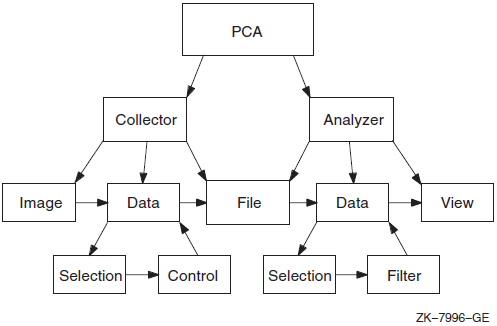
The Collector gathers many data kinds. In the Analyzer,you select which ones to analyze. Each data kind has one or more domains associated with it. For example, if you collected PC sampling, you can choose to view the following domains in the Analyzer: the program address, the call tree, the task, the task priority, and the task type. You can further restrict the data to be viewed with a filter. Any of the domains can be chosen and the value of the domain can be tested to be within a range of values. If it is within the range, then the selected domain value is passed along to be viewed. The general flow of control in PCA is shown in Figure 1.1, ''The PCA Model''.
The program counter (PC) of the I/O call
The file name
The virtual block number
Record size
I/O service name
Choosing the I/O data kind means you want to know the frequency of I/O calls. Choosing the Program Address domain indicates that you want to know where in the program the I/O calls occur. The Analyzer creates a view of the I/O data kind with the value of the PC from each I/O "record". The Analyzer uses the data to construct a view of the program, which shows where the I/O calls originate.
Filter selection differs from other selections because it is based on the values in the domain, not on the larger class of the data kind. For example, if you choose the I/O data kind with the Program Address Domain, set the filter for the Virtual Block Number domain, and specify a range of 1 to 5, the Program Address domain values then passed to the View are those which have Virtual Block Number domain values in the range of 1 to 5. In other words, you are asking where in my program are the I/O calls for Virtual Block number 1 to 5.
Selecting data kinds and domains can be thought of as progressively refining selected data from the data file before passing it on to be viewed.
View Selection
Histograms (Plot/Tables)
Source listings annotated with bars or numbers
Lists
Trees
Selecting the appearance of the view
Defining the granularity or size of each bucket
Defining the complete range
Setting the upper, lower, no zeros limits
Setting or canceling acceptable noncoverage (ANC)
Traversing the table
Expanding to source
Scaling
Scrolling
Selecting vertical versus horizontal views
Selecting numbers versus bars
Changing the title
1.4. Getting Started
This section uses as an example a FORTRAN program called PCA$PRIMES, which generates all the prime numbers in a given integer range. The program's source code has the file name PCA$PRIMES.FOR. The complete program is included in Appendix A, "Sample Programs" and is supplied with the PCA kit. (After installation, you can find PCA demonstration programs in the directory PCA$EXAMPLES.)
1.4.1. Using the Collector
The Collector gathers performance or test coverage data on applications programs as they run. In the example in the following sections, the Collector gathers program counter sampling data on the FORTRAN program PCA$PRIMES.
1.4.1.1. Invoking the Collector
- Compile the source file. Use the /DEBUG qualifier with a compilation command to create a Debug Symbol Table (DST) in the object module. The DST contains all of the symbol and line number information PCA needs to specify user program locations. Enter the following DCL command to compile the FORTRAN program PCA$PRIMES.FOR for use with the Collector:
$ FORTRAN/DEBUG PCA$PRIMES.FOR
This command creates the file PCA$PRIMES.OBJ. - Link the user program. The /DEBUG qualifier passes the DST information generated by the compiler to the executable image file where it can be accessed by the Collector. Type the following DCL command to link PCA$PRIMES.OBJ for running under Collector control:
$ LINK/DEBUG PCA$PRIMES.OBJ
- Run the program. Invoke the Collector on an image linked for debugging by defining the LIB$DEBUG logical to be PCA$COLLECTOR.EXE. This causes the OpenVMS image activator to invoke the Collector as a debugger. You can then enter Collector commands. Type the following commands to define the LIB$DEBUG logical:
$ DEFINE LIB$DEBUG SYS$LIBRARY:PCA$COLLECTOR.EXE
$ RUN PCA$PRIMES.EXE
1.4.1.2. Collecting the Data
PCAC> SET DATAFILE PCA$PRIMES
PCAC> SET PC_SAMPLING
PCAC> GO
%PCA-I-BEGINCOL, data collection begins 169 prime numbers generated between 1 and 1000 FORTRAN STOP %PCA-I-ENDCOL, data collection ends$
1.4.1.3. Exiting the Collector
To end the Collector session at any time prior to saying GO, or to suspend data collection, enter the EXIT command or press Ctrl/Z.
PCAC> SET DATAFILE/APPEND PCA$PRIMES.PCA
You can run your program without collecting data by entering the GO command with the /NOCOLLECT qualifier.
The Collector allows you to collect different kinds of data in the same collection run, but you should be cautious in doing so. Values may be distorted if different kinds of data are collected in the same collection run. The Collector provides informational messages warning about potential conflicts. Section 1.2, ''The Collector'' contains a listing of the different kinds of data you can collect.
1.4.2. Using the Analyzer
The Analyzer reads the performance data file written by the Collector and uses the data to produce histograms, tables, and other reports that help you evaluate your program's performance or coverage. In the example in the following sections, the Analyzer is used on the data file previously produced by the Collector to create histograms and tables, to display the source code and the summary page, and to print, file, and append Analyzer output.
1.4.2.1. Invoking the Analyzer
$ PCA PCA$PRIMES
Performance and Coverage Analyzer Version 5.0
PCAA>The
data file in the previous example, PCA$PRIMES.PCA, contains the performance or coverage data
and all symbol table information required by the Analyzer.$ PCA/COMMAND="SHOW DATAFILE; SHOW LANGUAGE" PCA$PRIMES.PCA
Performance and Coverage Analyzer Version 5.0
Performance Data File: SYS$DISK01:[SMITH]PCA$PRIMES.PCA;1
Language: FORTRAN
PCAA>In
this example, SHOW DATAFILE and SHOW LANGUAGE are executed before the Analyzer prompt
appears.1.4.2.2. Creating the Default Plot
After invoking the Analyzer and specifying the data file, you can enter a traverse command (NEXT, BACK, FIRST,CURRENT), and let the Analyzer default settings create a useful plot for you. The traverse commands walk you through your program's structure, pointing out the most significant portions of your application.
Entering the NEXT command at the first Analyzer prompt creates a source plot with the PC sampling data kind. A pointer is positioned at the line with the most data points in the routine with the most data points, that is, the place where the most PC samples were gathered and most of the time was spent. Subsequent NEXT commands traverse the program structure to show you the most-to-least significant line in the program.
The Analyzer supplies the default data kind. The default data kind is the last data kind collected by the Collector. If CPU sampling was the last data kind collected, then CPU sampling is the default data kind. You can change the default with the SET PLOT or PLOT commands.
1.4.2.3. Scrolling Through the Display on Your Terminal
A histogram or table is displayed on your terminal one page at a time. To see the next page, press the Return key. You can keep pressing Return to see successive pages until you reach the summary page. The summary page contains various summary statistics and lists all qualifiers and node specifications used to generate the Analyzer display. It can be more than one page. Section 1.4.2.4, ''Interpreting the Summary Page'' provides a detailed interpretation of the summary page. If you press Return at the end of the summary, the Analyzer brings you back to the first page of the histogram or table.
You can use the PAGE command to page through the histogram or table. You can also use the FIND command to look for a page with a specific label or line number.
When you have a histogram or table that you want to print or save in a file, you can do so with the PRINT, FILE, and APPEND commands (see Section 1.4.2.6, ''Printing, Filing and Appending Analyzer Output'').
1.4.2.4. Interpreting the Summary Page
Performance and Coverage Analyzer Page 2
Program Counter Sampling Data (27546 data points total) - "*"  PCA Version 5.0 20-OCT-2006 14:13:18
  PLOT Command Summary Information:
Number of buckets tallied: 17
PLOT Command Summary Information:
Number of buckets tallied: 17  Program Counter Sampling Data - "*"
Data count in largest defined bucket: 27477 99.7%
Program Counter Sampling Data - "*"
Data count in largest defined bucket: 27477 99.7%  Data count in all defined buckets: 27539 100.0%
  Data count not in defined buckets: 0 0.0%
  Portion of above count in P0 space: 0 0.0%
  Number of PC values in P1 space: 0 0.0%
  Number of PC values in system space: 0 0.0%
  Data points failing /STACK_DEPTH or /MAIN_IMAGE: 7 0.0%
  Total number of data values collected: 27546 100.0%
  Command qualifiers and parameters used:
  Qualifiers:
/PC_SAMPLING /DESCENDING /NOMINIMUM /NOMAXIMUM
/NOCUMULATIVE /NOSOURCE /ZEROS /NOSCALE /NOCREATOR_PC
/NOPATHNAME /NOCHAIN_NAME /WRAP /NOPARENT_TASK /NOKEEP /NOTREE
/FILL=("*","O","x","@",":","#","/","+")
/NOSTACK_DEPTH /MAIN_IMAGE
Node specifications:
PROGRAM_ADDRESS BY MODULE
No filters are defined
Qualifiers:
/PC_SAMPLING /DESCENDING /NOMINIMUM /NOMAXIMUM
/NOCUMULATIVE /NOSOURCE /ZEROS /NOSCALE /NOCREATOR_PC
/NOPATHNAME /NOCHAIN_NAME /WRAP /NOPARENT_TASK /NOKEEP /NOTREE
/FILL=("*","O","x","@",":","#","/","+")
/NOSTACK_DEPTH /MAIN_IMAGE
Node specifications:
PROGRAM_ADDRESS BY MODULE
No filters are defined  PCAA>
PCAA>Not all of the lines shown in the example appear in all summary pages. For example, the summary page does not display the lines showing the number of PC values in P0, P1, or system space unless you have tallied program addresses.
Performance and Coverage Analyzer Page 3
I/O System Service Calls (3581 data points total) - "*"
Page Fault Program-Counter Data (121 data points total) - "O"
Program Counter Sampling Data (27546 data points total) - "x"
PCA Version 5.0 20-OCT-2006 14:15:32
PLOT Command Summary Information:
Number of buckets tallied: 17
I/O System Service Calls - "*"
Data count in largest defined bucket: 3581 100.0%
Data count in all defined buckets: 3581 100.0%
Data count not in defined buckets: 0 0.0%
Portion of above count in P0 space: 0 0.0%
Number of PC values in P1 space: 0 0.0%
Number of PC values in system space: 0 0.0%
Data points failing /STACK_DEPTH or /MAIN_IMAGE: 0 0.0%
Total number of data values collected: 3581 100.0%
Command qualifiers and parameters used:
Qualifiers:
/IO_SERVICES /DESCENDING /NOMINIMUM /NOMAXIMUM
/NOCUMULATIVE /NOSOURCE /ZEROS /NOSCALE /NOCREATOR_PC
/NOPATHNAME /NOCHAIN_NAME /WRAP /NOPARENT_TASK /NOKEEP /NOTREE
/FILL=("*","O","x","@",":","#","/","+")
/NOSTACK_DEPTH /MAIN_IMAGE
Node specifications:
PROGRAM_ADDRESS BY MODULE
Filter definitions:
Filter F1:
RUN_NAME = 2
Page Fault Program-Counter Data - "O"
Data count in largest defined bucket: 46 38.0%
Data count in all defined buckets: 121 100.0%
Data count not in defined buckets: 0 0.0%
Portion of above count in P0 space: 0 0.0%
Number of PC values in P1 space: 0 0.0%
Number of PC values in system space: 24 19.8%
Total number of data values collected: 121 100.0%
Qualifiers applied to this datakind:
/NOCUMULATIVE /NOSTACK_DEPTH /NOPARENT_TASK /NOCREATOR_PC
/NOMAIN_IMAGE
Filter definitions:
Filter F1:
RUN_NAME = 1
Program Counter Sampling Data - "x"
Data count in largest defined bucket: 27477 99.7%
Data count in all defined buckets: 27539 100.0%
Data count not in defined buckets: 0 0.0%
Portion of above count in P0 space: 0 0.0%
Number of PC values in P1 space: 0 0.0%
Number of PC values in system space: 0 0.0%
Data points failing /STACK_DEPTH or /MAIN_IMAGE: 7 0.0%
Total number of data values collected: 27546 100.0%
Qualifiers applied to this datakind:
/NOCUMULATIVE /NOSTACK_DEPTH /NOPARENT_TASK /NOCREATOR_PC
/MAIN_IMAGE
No filters are defined
| Data kind lines. Each line of this header information names one of the data kinds plotted, in the order that they were plotted. |
| Summary information by data kind. The summary information is repeated for each data kind, and is presented in the order that they were plotted. |
| Qualifier information. This list includes all qualifiers used by the Analyzer. Subsequent qualifier information lists only those applied to the data kind. |
| Filters applied to this data kind. This line includes only the filters that were defined for this data kind. |
| Qualifiers applied to this data kind. This list includes only the qualifiers applied to this data kind. |
Information that does not vary among the data kinds (such as the number of buckets, the qualifier list, and node specification) is only displayed once.
1.4.2.5. Viewing the Currently Active Plot
The plot or table resulting from the last PLOT or TABULATE command you entered is known as the currently active plot. The currently active plot is the source of all default qualifiers and parameters for a subsequent PLOT or TABULATE command. Use the SHOW PLOT command to view all the attributes of the currently active plot.
1.4.2.6. Printing, Filing and Appending Analyzer Output
The PRINT, FILE, and APPEND commands act on the output from the last PLOT, TABULATE, INCLUDE, EXCLUDE, LIST or traverse command you entered. You can use PRINT, FILE, APPEND commands to print or file raw performance data in addition to histograms and tables. Also, with the FILE/DDIF command, you can store your output in a DDIF file to process for a specified printing device.
PCAA> PRINT %PCA-I-FILQUE, print file queued to SYS$PRINT PCAA>To be notified on your terminal when the print job has completed, use the /NOTIFY qualifier with the PRINT command. No other qualifiers are accepted.
PCAA> FILE OUTFILE %PCA-I-CREFILE, creating file SYS$DISK01:[LEE]OUTFILE.PCALIS;1 PCAA>
PCAA> APPEND %PCA-I-APPFILE, appending to file SYS$DISK01:[LEE]OUTFILE.PCALIS;1 PCAA>
1.4.2.7. Stopping Terminal Output or Exiting the Analyzer Session
To stop the Analyzer's terminal output, such as long output from a SHOW or LIST command, press Ctrl/C. The Analyzer aborts the current output operation and prompts for a new command.
To end the Analyzer session, enter the EXIT command or press Ctrl/Z.
Chapter 2. Using the Collector
This chapter explains how to invoke the Collector, how to set up the Collector environment, and how to specify and filter the data you want to collect on your application's performance.
2.1. Overview
Invoke the Collector by compiling, linking and running your application.
Specify the name of the performance data file.
Specify the data kinds to collect.
Select the language of your application.
Name the collection run.
Type GO to start the collection run and store the data in the performance data file.
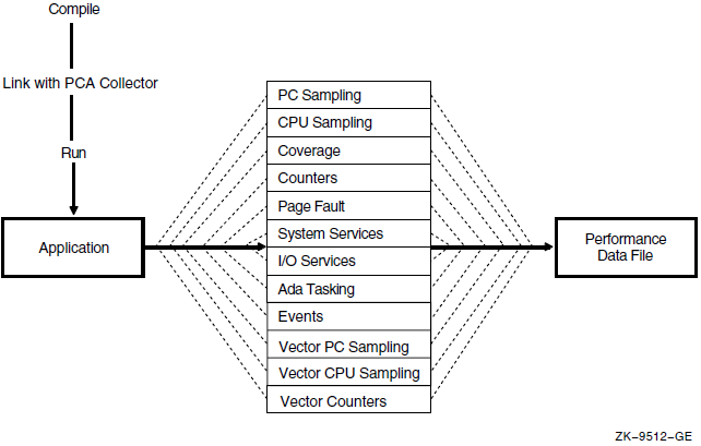
Figure 2.1, ''The PCA Collector'' shows how the Collector interacts with your application to collect data.
2.2. Invoking the Collector
$ LINK/DEBUG PCA$PRIMES.OBJ
$ DEFINE LIB$DEBUG PCA$COLLECTOR.EXE
$ RUN PCA$PRIMES.EXE
                         PCA Collector Version 4.6
PCAC>To
return to the debugger, deassign the logical name LIB$DEBUG, as
follows:$ DEASSIGN LIB$DEBUG
$ RUN PCA$PRIMES.EXE
OpenVMS Debugger Version 7.0
DBG>When collecting coverage data, use the /NOOPTIMIZE qualifier during compilation.
2.3. Specifying the Performance Data File
PCAC> SET DATAFILE PCA$PRIMES_PC_SMPL
If you do not specify a data file,the Collector names the data file after the executable image file of the program you are measuring with a default file type of .PCA.
To direct the gathered data to a new data file with each run,enter a new SET DATAFILE command for each collection run.
Appending a New Data Collection to an Existing File
PCAC> SET DATAFILE/APPEND/EXECUTABLEThis example sets the data file to the default data file. When using the /EXECUTABLE qualifier, omit the file specification parameter.
2.4. Specifying Data Collection
When you invoke the Collector and name the data file,you must specify the kinds of data you want to gather.
PC Sampling
CPU Sampling
Coverage
Counters
Page fault
System services
I/O services
Ada tasking
Events
Vector PC sampling
Vector CPU sampling
Vector counters
By default, PCA collects PC sampling and stack data when you enter a GO command without specifying a data kind.
| Set PC_Sampling | (see Section 2.4.1, ''Program Counter Sampling Data: System Time'') |
| Set PCU_Sampling | (see Section 2.4.2, ''Program Counter Sampling Data: CPU Time'') |
| Set Page_Faults | (see Section 2.4.1.4, ''Interpreting Page-Faulting Data'') |
| Set Services | (see Section 2.4.6, ''System Services Data'') |
| Set IO_Services | (see Section 2.4.7, ''Input/Output Data'') |
| Set Tasking | (see Section 2.4.8, ''Tasking Data'') |
2.4.1. Program Counter Sampling Data: System Time
PCAC> SET PC_SAMPLINGThe Collector samples the PC by setting up an asynchronous system trap (AST) timer routine in supervisor mode. By default, the AST timer routine is activated every 10 milliseconds. Each time the routine is activated, the Collector retrieves the current PC value for output to the data file. Because the timer operates in supervisor mode, it samples the PC in all user-mode and user AST-mode that your program executes. The Collector cannot collect data on programs that run in other modes.
PC sampling data collection is efficient. The extra overhead of gathering this data is typically no more than 5 percent of the total run time of the user program. However, run times of a minute or more are required to gather enough PC values for statistically significant results. You can gather at most 100 values per second, and you usually need to gather thousands of values to get significant results.
2.4.1.1. PC Sampling Data Distortion
PC sampling provides correct and repeatable results if the Collector supplies enough PC values for statistically significant results. When collecting PC values under ideal conditions, the chances of finding the PC in a given address range is proportional to the amount of time the program actually spends in that address range. However, when less than ideal conditions exist, the results of PC sampling may be distorted. This section discusses those situations that can distort PC sampling data and lead you to draw incorrect conclusions about the behavior of your program.
The overall system load at the time of collection affects the number of program counter values the Collector gathers, because program execution slows down as more demands are made on the system CPU. When program execution slows, the 10-millisecond timer (which is relatively unaffected by the CPU load) gathers more PC values per program run than when your system is lightly loaded and processing faster. The actual number of PC values collected is not important as long as the number is large enough to establish a representative sample. Only the proportion of PC values found in a given address range is significant and repeatable.
A less than ideal condition exists when the system load changes markedly during the PC sampling session. This condition may force the program you are measuring to share the system with a CPU-intensive process. This would cause the program to run more slowly in real time, produce more 10-millisecond ticks, and collect a greater number of PC values. Now, consider that the other process may terminate at some point through the PC sampling run. If this occurs, then the rest of the PC sampling run executes at full speed, experiences fewer 10-millisecond ticks, and collects fewer PC values than it did before the other process terminated. Under these conditions, the PC sampling data would be misleading because the program was not run on an evenly loaded system. There could be a skew of PC sampling data toward the beginning of the run.
Synchronizing your code with the 10-millisecond timer can also cause PC sampling data distortion. For example, if your program sets up a user-mode timer AST routine, then that routine normally gains control as soon as the Collector's supervisor-mode timer AST routine runs to completion. The AST routine starts early in the Collector's timer interval and probably finishes before the next 10-millisecond tick occurs. Therefore, no PC values are likely to be collected from such an AST routine, and you may wrongly conclude that no time is consumed in that routine. An example of this situation is an Ada multi-tasking program that is time slicing at every 10 milliseconds.
2.4.1.2. Interpreting System Service Wait Times
Interpreting system service wait times can also be deceiving. When your program calls a system service that runs in executive or kernel mode, the PC points to the first byte following a change-mode instruction in the system service vector in P1 space. However, as long as the system service is running in that higher mode, the Collector's supervisor-mode timer AST routine cannot gain control. When the higher-mode code has finished executing, the Collector's AST routine gains control and collects only one PC value, even if many 10-millisecond ticks occur in that time frame. Therefore, the amount of CPU time consumed in system services may not be properly represented in the PC sampling data.
2.4.1.3. Interpreting I/O Services Wait Times
In comparison to system service wait times, I/O services wait times are properly represented in PC sampling data. The CPU time used by the I/O system services may be under represented, but once the physical I/O operation is queued or started, the Collector's timer AST routine can continue to collect PC values. Therefore, I/O-bound programs may result in large numbers of PC values occurring in P1 space. These values represent I/O system service wait times.
Under some circumstances, I/O wait times should be evaluated cautiously. For example, if your program is accessing an overloaded disk, much of the wait time may be due to competition from other processes accessing the same device. In such cases, the best way to reduce program I/O wait time is to reduce the load on that disk, perhaps by spreading its files over several disks. Before you decide to code your program to make it faster, you should consider both the internal and external factors that can be causing poor I/O performance.
Because terminals are inherently slow devices, terminal I/O is likely to cause many PC values to be collected in P1 space. A terminal-bound application can easily spend 80 to 90 percent of its time waiting for the terminal. Collecting many PC values in P1 space is a normal characteristic of terminal-bound programs.
2.4.1.4. Interpreting Page-Faulting Data
PC sampling data measures page faulting time in addition to CPU and I/O time. When a page fault occurs, the Collector gathers the PC value of the instruction that caused the page fault. If you find a big PC sampling peak in a routine or in a code segment, the peak could be due to page faulting rather than to CPU usage. If you are in doubt about the PC data, collect page fault data or collect CPU sampling data to see if that can explain the PC sampling peak in that code segment.
2.4.1.5. Collecting PC Sampling Data and Other Data in the Same Run
You can collect different kinds of data in the same collection run. However, some kinds of data impose a high collection overhead that can substantially alter the run-time behavior of your program. For this reason, the Collector provides an informational message warning about possible conflicts. For example, execution counters can slow your program down several hundred times. If you try to collect execution counts and PC sampling data at the same time, the overhead of collecting execution counts may make the PC sampling data meaningless.
Although you should avoid collecting PC sampling data and execution count data at the same time, there are exceptions. For example, an execution counter that is "hit" only half a dozen times in a long collection run may have no appreciable effect on the PC sampling process.
Usually, you can collect page fault data and PC sampling data at the same time with little or no distortion in either kind of data. However, avoid collecting system services data, I/O data, CPU sampling data, execution counts,or test coverage data at the same time that you collect PC sampling data.
2.4.2. Program Counter Sampling Data: CPU Time
PCAC> SET CPU_SAMPLING
There are many external factors that can affect the behavior of a program in relation to the system clock (for example, page faulting and system service wait time, including I/O wait time). These conditions make it difficult to determine whether the program counter contains a specific location because of the structure of the program's algorithm or because of other external factors occurring in that interval. Under these conditions, sampling the PC values based on the CPU time is more effective and reproducible because the effects caused by contending processes are eliminated.
2.4.3. Test Coverage Data
If you want to see which parts of your application are covered or not covered by your test suite, use the SET COVERAGE command. You must use node specifications to specify program locations on which to place breakpoints so that test coverage data or execution counts can be gathered for that area of the program. Node specifications refer to those elements of your application that can be defined as a program address, a module, a routine, a code path, or a line.
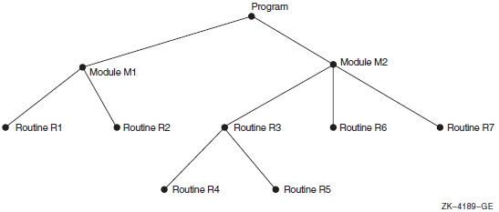
Figure 2.2, ''A Program Represented as a Tree'' depicts the different elements of a program as a tree structure. Many of the examples used in the following sections refer to its modules and routines by name.
PCAC> SET COVERAGE/STACK_PCS PROGRAM BY CODEPATH
By default, the Collector removes each breakpoint the first time the code executes. This allows the program to run faster because it does not collect counts at locations that have already been covered. Therefore, frequently executed code runs at full speed after the first execution.
The complete syntax of node specifications, as used with the SET COUNTERS, SET COVERAGE, and SET EVENT commands, is shown in Table B.3, ''Node Specification Parameter Syntax''.
2.4.3.1. Codepaths
When you use the SET COVERAGE command, the most useful node specification is one with a BY CODEPATH clause. This nodespec causes the Collector to examine the program's object code in order to find all relevant codepaths. The term codepath is any piece of object code that the executing program enters only at the beginning (at the first instruction) and exits only at the end.
The codepath search starts at all entry points and labels. The Collector puts breakpoints at the entry points of the routines and at all possible destinations of conditional branches. In this regard, you can think of the codepath source as being a basic block within a high level language. In the Analyzer, you can plot or tabulate the collected data to see which codepaths are not covered by your tests.
PCAC> SET COVERAGE MODULE M2 BY CODEPATHSimilarly, the following command places test coverage counters on all codepaths in the entire program:
PCAC> SET COVERAGE PROGRAM_ADDRESS BY CODEPATHBecause the MACRO assembler does not provide adequate symbol table information, the Collector may not be able to find all codepaths in MACRO programs. To minimize this problem, you should declare all MACRO routines with .ENTRY directives. Even then, constructs such as indexed jump instructions or passing code addresses as parameters may cause codepaths to be missed.
PCAC> SET COVERAGE ROUTINE R6, ROUTINE R7, MODULE M1 BY ROUTINE
PCAC> SET COVERAGE PROG BY LINE, PROG BY CODEThis covers the union of addresses specified in the nodespec but may create an inordinate number of buckets.
PCAC> SET COVERAGE/UNTIL:3 ROUTINE FINDSUM BY CODEPATH
When compiling your program to gather coverage data, use the/NOOPTIMIZE qualifier to prevent the compiler from optimizing code and gathering incorrect results.
2.4.3.2. Modules
PCAC> SET COVERAGE MODULE M1 BY ROUTINE
If the subtree with Module M1 as its root has routine nodes for both R1 and R2, coverage breakpoints are placed on those two routine nodes, but not on root node Module M1.
2.4.3.3. Routines
2.4.3.4. Lines
PCAC> SET COVERAGE ROUTINE R3 BY LINEYou can also use the PROGRAM_ADDRESS BY LINE nodespec. Measuring test coverage at that many program locations is reasonable because test coverage data is collected only once for each line.
You can use the SEARCH and TYPE commands to display specific lines, or a range of lines. See Section 4.7.4.1, ''Viewing Displays with TYPE and SEARCH Commands'' for information on these commands.
2.4.3.5. Path-Name Qualification
PCAC> SET COVERAGE ROUTINE M1\R2 BY LINEIf a routine is nested within other routines, further qualification may be required in the routine's path name. Routine R4, for example, is nested within Routine R3, which is nested in Module M2. Its full path name is M2\R3\R4.
Specifying Path Names for Source Lines
R4\%LINE 25, R3\R4\%LINE
25, or M2\R3\R4\%LINE 25. However, specifying only the module
name and line number is sufficient because line numbers are always unique within a separately
compiled module. For example:PCAC> SET COVERAGE LINE M2\%LINE 25
2.4.3.6. Collecting Coverage Data from Multiple Test Runs
PCAC> SET DATAFILE/APPEND MY_DATAFILE.PCA PCAC> SET COVERAGE/PREVIOUS PROGRAM_ADDRESS BY CODEPATH
The /PREVIOUS qualifier causes the Collector to measure coverage at each designated program location only once during the entire set of program executions (collection runs). If a location has been covered in a prior execution, the Collector does not attempt to measure coverage of that location in subsequent executions of the program.
If the SET DATAFILE command creates a new data file, it then places test coverage breakpoints on all program locations that you specified on the SET COVERAGE command. When the collection run ends, all breakpoint locations not hit (or not hit n times if /UNTIL:n was also specified) are recorded in the data file as not covered.
If the SET DATAFILE command finds an existing file, then the breakpoint locations recorded by the previous collection run (those that were requested but not hit) are used. In this case, if you specify node specifications, they are ignored. When the collection run ends, all breakpointl ocations still not hit are once again recorded in the data file as not covered. Thus, each collection run starts with the breakpoint locations remaining from the previous collection run and passes on a reduced breakpoint table to the next collection run.
If you intend to use the Analyzer MERGE/ANC command (see Section 3.4.1, ''Merging PCA Performance and Software Performance Monitor (SPM) Files'') to write acceptable noncoverage information to a table, use the /ANC qualifier. This qualifier instructs the Collector to save the codepaths of the current version of the program for comparison with codepaths from another version of the program. This information is comprised of all codepath information in the modules that were specified by the nodespec in the SETCOVERAGE/ANC command. The Analyzer can tell which routines have changed from this saved information. See Section 3.6, ''Using Acceptable Noncoverage (ANC)'' for information on acceptable noncoverage (ANC).See Section 4.5, ''Determining Acceptable Noncoverage (ANC)'' for an example of collecting, merging and setting ANC data.
2.4.3.7. Gathering Test Coverage Without Optimization
When gathering information on how completely a given set of test data covers your program, you may find it helpful to first compile your program with the /NOOPTIMIZE qualifier. Compiling the program without optimization makes the program run slower, but may make it easier to relate the coverage points in the object module back to the original source code. If you measure test coverage over fully optimized code, then simple one-to-one correspondence between the coverage points in the optimized object code and the constructs in your source program may be lost.
2.4.4. Execution Count Data
The SET COUNTERS command determines the exact number of times that various parts of your program execute by placing breakpoints at specified program locations. Each time a breakpoint executes, the Collector records a count for that location. The Collector lets you specify these locations either individually or collectively. For example, an individual location could be line 6 of routine FINDSUM in your program, whereas a type of program locations could be every routine in the whole program or every line in a given routine.
PCAC> SET COUNTERS LINE FINDSUM\%LINE 6The nodespec FINDSUM\%LINE 6 specifies an individual program location for an execution counter. In the next example, the PROGRAM_ADDRESS BYROUTINE nodespec causes execution counters to be placed on every routine in the entire program:
PCAC> SET COUNTERS PROGRAM_ADDRESS BY ROUTINE
Note
Counting the number of times that program locations execute greatly increases CPU overhead. Therefore, you should be selective in using execution counters.
Placing an execution counter on every line in a program may make the program run a hundred times slower. Place execution counters at the entry point to each routine in your program, or for all lines in one routine, or for only strategic program locations.
It is practical to use execution counters when you need more exact data than you can get from PC sampling. Because execution count results are repeatable (provided the program and its input are fixed), useful data can be collected in short collection runs.
2.4.5. Page Fault Data
The address of the instruction that caused the fault
The faulting virtual address
The current CPU time
PCAC> SET PAGE_FAULTS
Collecting page fault data alters your program's page faulting behavior. The Collector requires some code and data to collect page fault data and therefore produces paging of its own. This reduces your program's working set, which increases the program's paging. This usually has little or no effect on the sites of the page faulting peaks in your program; the small disruptions introduced by the Collector can usually be ignored when you are trying to discover where your program is producing the most page faults.
Distortions introduced by collecting page fault data and other data at the same time can be significant. The process of collecting these other kinds of data may in itself cause page faulting, which distorts the page fault data. Avoid collecting call stack return addresses when collecting page fault data because the Collector can affect your program's page faulting behavior as it traverses the call stack. Call stack return addresses cannot be collected for the page fault data itself, but can be collected for other kinds of data during the run.
PCA supports this command on both OpenVMS VAX and OpenVMS Alpha.
2.4.6. System Services Data
The system service index
The PC address of the system service call
The current CPU time
PCAC> SET SERVICES
PCA supports this command on both OpenVMS VAX and OpenVMS Alpha.
For more information on system services and a list of the available system services, see the VSI OpenVMS System Services Reference Manual.
2.4.7. Input/Output Data
PCAC> SET IO_SERVICES
The SET IO_SERVICES command measures several Record Management Services (RMS). See Appendix B, "PCA Reference Tables" for a listing of both RMS and non-RMS services measured by this command. For more information on RMS services, see the VSI OpenVMS Record Management Services Reference Manual.
The I/O system service index
The PC address of the I/O call
The current CPU time
The file name
The physical I/O read count
The physical I/O write count
The file access block (FAB)
The record access block (RAB)
PCA supports this command on both OpenVMS VAX and OpenVMS Alpha.
2.4.8. Tasking Data
PCAC> SET TASKING
The context switch
The task priority
The task type
The PC value of the address where the task was created
The CPU time
The parent task
PCA supports this command on both OpenVMS VAX and OpenVMS Alpha.
2.4.9. Events Data
You can filter your data so that the Analyzer creates histograms or tables using only data from a specified phase of your program. Place event markers in the datafile using the Collector SET EVENT command. An event marker is a record that the Collector inserts into the data file whenever control passes to a specified program location during program execution.
PCAC> SET EVENT COMPUTE LINE M1\R2\%LINE 25In this example, the event name is COMPUTE and the event breakpoint location is line 25 of Routine R2 in Module M1. Whenever line 25 executes, an event marker for event COMPUTE is written to the data file. If you specify more than one breakpoint location for the event COMPUTE, execution of any of the designated locations would mark that event in the file.
You can use event markers to limit analysis of performance data to data collected between any two events occurring in your program's execution. The event marked is the execution of code at that program location.
The SET EVENT command causes the Collector to insert breakpoints at specified program locations. When the breakpoint location executes, all currently accumulated data is written to the data file followed by a time-stamped event marker record. The event marker record signifies that the indicated event occurred. You must specify an event name for each event. The Collector records all event names in your data file. Event markers, in effect, partition the collected data by time.
For example, if your program consists of three main phases—an input phase,a compute phase, and an output phase, executed in that order—you may want to look at the data from only one of these phases. If you want to investigate how often your program calls a particular utility routine during the compute phase of your program, place an event marker at the beginning of the compute phase and at the beginning of the output phase. Then, you can examine the data that is collected between these event markers. Data gathered between two event markers is associated with the event name given to the first of the two markers.
2.4.10. Collecting Vector Instruction Data
SET VCOUNTERS
SET VCPU_SAMPLING
SET VPC_SAMPLING
This section summarizes each of these commands. Chapter 5, "Using VAX Vectors with PCA" contains a complete discussion of using VAX Vectors with PCA.
2.4.10.1. Vector Program Counter Sampling Data
The SET VPC_SAMPLING Collector command lets you collect PC values for random vector instructions based on the wall clock. The collected data lets you determine the scalar/vector parallelism throughout your entire program.
When you collect vector PC samples, you set a sampling interval timer that includes all idle time associated with the current run of the program. This form of sampling shows you where the time is being spent in the program with little cost to the time of actually running the program.
2.4.10.2. Vector CPU Time Data
The SET VCPU_SAMPLING Collector command allows you to collect PC values for random vector instructions based on the processor clock. The collected data lets you determine the scalar/vector parallelism throughout your entire program.
When you collect vector CPU samples, you set a sampling interval timer that includes only the time when the program is actually running the processor. This form of sampling allows you to focus on the particular area of the program's algorithm where the time is being spent, and not on the areas where outside influences consume time.
2.4.10.3. Vector Instruction Execution Count Data
PROGRAM ADDRESS by VINSTRUCTION
MODULE module-name by VINSTRUCTION
ROUTINE routine-name by VINSTRUCTION
2.4.11. Collecting PC Values from the Call Stack
For some forms of data collection, the Collector records the current value of the program counter, along with the other data collected. The Analyzer uses the program counter to associate the collected data with the particular module, routine, line, or other program unit that generate the data.
Sometimes the value of the program counter may not be the most meaningful program address to collect. For example, if you gather I/O data on your FORTRAN program, the PC values of all the I/O system service calls are within the address range of the FORTRAN Run-Time Library. What you really need to know is what sections of your FORTRAN program are causing the I/O calls. To discover what program code is calling the Run-Time Library, you must gather all subroutine return addresses stored on the stack for each collected data point.
PC sampling data
CPU sampling data
System services data
I/O services data
Exact execution counts
Test coverage data
Vector PC sampling data
Vector CPU sampling data
Vector counters data
PCAC> SET STACK_PCS
Collecting this data adds to the amount of data gathered and to the processing overhead of gathering the data. However, you can gather exactly the data you need and minimize PCA's overhead by selectively collecting desired data kinds with the /STACK_PCS qualifier.
2.4.11.1. Collecting Stack PCs by Data Kind
Call Stack return addresses can be gathered selectively by data kind with the /STACK_PCS qualifier. The /STACK_PCS qualifier allows you to collect only the data that you need, thus minimizing PCA's overhead.
The /STACK_PCS qualifier causes the collection of stack PC values. The /NOSTACK_PCS qualifier prevents the collection of stack PC values.
PCAC> SET CPU_SAMPLING/NOSTACK_PCS
PCAC> SET IO_SERVICE/STACK_PCS PCAC> CANCEL IO_SERVICE PCAC> SET IO_SERVICEYou can collect stack PC values for all nodespecs of a measurement,or for none. If you enter the following command sequence, then stack PC values are not collected:
PCAC> SET COUNTERS/STACK_PCS MODULE A BY LINE PCAC> SET COUNTERS/NOSTACK MODULE B BY LINE PCAC> SET COUNTERS MODULE A BY LINEThe SET STACK_PCS command overrides all previously set /NOSTACK_PCS qualifiers and causes a new default of /STACK_PCS. The CANCEL STACK_PCS command overrides all previously set /STACK_PCS qualifiers and causes a new default of /NOSTACK_PCS. For information on data kind collection in vector applications, see Chapter 5, "Using VAX Vectors with PCA".
2.5. Selecting the Language of Your Application
The language setting determines how PCA parses symbol names in command input. If the language is set to C, PCA treats symbol names as case sensitive. If the language is set to anything other than C or C++, symbol names are assumed to be case insensitive.
PCAC> SET LANGUAGE C
This command changes the language setting to C. Symbol names are then parsed by the C language rules.
2.6. Naming the Collection Run
Each program execution run under Collector control is called a collection run. The data collected from each collection run is recorded separately in the performance data file. Collection run numbers are assigned sequentially by the Collector, starting at 1.
PCAC> SET RUN_NAME name-of-run
If name-of-run does not start with an alphabetic character, you must enclose it in quotation marks.
If you assign the same collection run name to more than one collection run in the same data file, data from all those runs passes the filter specified by that name. Thus, you can assign the same collection run name to a whole group of collection runs when you intend to filter that group of runs as a unit in the Analyzer.
If you do not use the SET RUN_NAME command, you get a null run name; the Collector assigns a number as a run name. To show collection run names, use the SHOW RUN_NAME command.
2.7. Starting and Terminating Data Collection
After you invoke the Collector and optionally set the data file and collection type, enter the GO command to start data collection.
To stop a Collector session before you enter the GO command, enter the EXIT command or press Ctrl/Z. If the data collection has already started, you cannot enter an EXIT command; you must press Ctrl/Y to stop the collection run.
If you press Ctrl/Y, do not use the DCL STOP command immediately afterward. If Ctrl/Y interrupts the Collector when the Collector is executing supervisor-mode code, a subsequent STOP command may cause a supervisor-mode exception that kills your entire process and logs you out. To avoid this, execute another program after pressing Ctrl/Y, or type EXIT. The Collector's exit handlers then successfully close out the data collection.
To stop Collector output to your terminal, such as SHOW command output, press Ctrl/C. The Collector aborts the command and returns to DCL level.
To run your program without collecting data, use the /NOCOLLECT qualifier with the GO command.
2.8. Using Collector Command Procedures
If you repeatedly enter the same group of commands to the Collector, then place those commands into a command procedure. This makes command entry more efficient and less error prone.
A command procedure is a text file of commands that substitute for an interactively entered sequence of commands. The default file type is .PCAC. Add SET VERIFY to the procedure to view the commands as they are executed from the procedure.
When the Collector encounters a GO command in a command procedure, it starts collecting data and does not accept additional commands from the terminal or from the command procedure. If a command procedure does not contain a GO command, the Collector interactively prompts for further commands after executing the commands in the command procedure.
When the Collector encounters an EXIT command in a command procedure, that command procedure terminates and control returns to the command stream (either the terminal or a previous command procedure) that invoked the command procedure.
$ DEFINE PCAC$INIT SYS$LOGIN:COLLECTOR_STARTUP.PCAC
SET DATAFILE/APPEND PRIMES_IO ! Append data to existing file SET IO_SERVICES ! Collect I/O services data GO ! Start collection
2.9. Using Collector Logical Names
The Collector checks for a number of logical names which, if defined, modify the activity of the Collector in various ways. These names perform functions such as defining input and output streams and defining the name of the performance data file to use. In Section 2.8, ''Using Collector Command Procedures'', PCAC$INIT was used to define an initialization file. As a convenience, use logical names rather than repeated commands to pass information to the Collector.
|
PCAC$DATAFILE |
PCA$RUN_NAME |
|
PCA$INHIBIT_MSG |
PCAC$INIT |
|
PCAC$INPUT |
PCAC$OUTPUT |
|
PCAC$DECW$DISPLAY |
For a more detailed description of these logical names, see Table B.4, ''Collector Logical Names''.
2.10. Gathering Shareable Image Data
Note
There are two classes of shareable images: those that are user written, and those that are provided. The Analyzer can report symbolically only on user-written shareable images. See the VSI OpenVMS Linker Utility Manual for more information on shareable images.
The Collector writes all shareable image names and address ranges to the performance data file. The Analyzer uses this information to report on each shareable image.
User-Written Shareable Images
- Compile all sources for the shareable image with /DEBUG to gather performance data on a shareable image. To do symbolic performance analysis on the shareable image, first compile the sources:
$ FORTRAN/DEBUG SHARE
In this example, MAIN.FOR is the source file for your main image, and SHARE.FOR is the source file for the shareable image to be called by other programs. Assume that SHARE.FOR has a single universal symbol called SHARED_ROUTINE, which isa routine called from the main program MAIN.FOR.
- Enter LINK/SHAREABLE/DEBUG to create a version of the shareable image that contains the DST information the Collector needs and enter the universal symbol:
$ LINK/SHARE/DEBUG SHARE,SYS$INPUT/OPTION- _$ UNIVERSAL=SHARED_ROUTINE Ctrl/ZThis command builds the shareable image SHARE.EXE in your current directory.
- Link the program /DEBUG to link the programs that use the shareable image. Because it is a shareable image, you cannot run SHARE.EXE directly. Instead, you have to link your main image against it, then point the logical name SHARE to your copy of SHARE.EXE:
$ LINK/DEBUG MAIN,SYS$INPUT/OPTION SHARE.EXE/SHARE Ctrl/Z $ DEFINE SHARE SYS$DISK:[]SHARE.EXEPoint LIB$DEBUG to PCA Collector:$ DEFINE LIB$DEBUG PCA$COLLECTOR
- Run the programs that use your shareable image, as follows:
$ RUN MAIN PCA Collector Version 4.6 PCAC> - Enter the SET DATAFILE/SHAREABLE=img-name command. This command specifies the shareable image to be measured.(The /SHAREABLE=(img-name,dst-file) form of the /SHAREABLE qualifier is supported, but only for the sake of compatibility with PCA Version 1.0.) When you get the Collector prompt, enter the SET DATAFILE command:
PCAC> SET DATAFILE/SHAREABLE=SHARE MY_DATAFILE.PCA
SHARE is the name of the shareable image to be measured, and MY_DATAFILE.PCA is the file specification for the performance data file.
The Collector creates the performance data file, extracts the required symbol table information from the shareable image, and writes it to the data file. The Collector then prompts for additional commands.
Specify your remaining data collection commands and enter a GO command to start the data collection. After the collection run ends, you can process the performance data by running the Analyzer.
You can measure the performance of one shareable image averaged over many executions of different programs. Use the /APPEND qualifier to collect data from several program executions into one data file.
Chapter 3. Using the Analyzer
This chapter describes the Analyzer, explains the steps you must follow to use the Analyzer, and provides examples of tasks you can perform while using the Analyzer.
3.1. Overview
Invoke the Analyzer, which then reads the performance datafile that the Collector has built.
View the performance data results as tabular and graphical reports, filtering and refining the data to get a more detailed view.
Analyze and pinpoint the bottlenecks in your application or evaluate the thoroughness of your testing environment.
Each of these steps is described fully in this chapter.
Performance histograms showing how much time or other resource is consumed by various parts of your program
Tables showing information in the form of raw data counts and percentages
Annotated source listings showing performance or coverage data
Histograms and tables for other data domains, such as the number of calls per system service, or the amount of I/O per file used by your program
Listings of your raw performance data
Dynamic call trees that show the frequency of each call chain
3.2. Invoking the Analyzer
$ PCA PCA$PRIMES

         Performance and Coverage Analyzer Version 5.0

PCAA>
The data file in the previous example, PCA$PRIMES.PCA, contains the performance or coverage data and all symbol table information required by the Analyzer.
See Chapter 1, "Introduction" for complete information on invoking the Analyzer, creating the default plot, scrolling through your display, interpreting the summary page, and printing, filing, and appending Analyzer output.
3.3. Generating Histograms and Tables
The PLOT and TABULATE commands display performance and coverage data in an understandable form. The PLOT command produces performance histograms that plot the distribution of resource usage over your program or over other data domains. The TABULATE command presents the same information in the form of tables so you can see the actual data counts, instead of scaled histogram bars.
The PLOT and TABULATE command qualifiers specify the kind of data to analyze, and the format and display of the output.
When you enter a PLOT command, use the qualifiers to specify what kind of data to tally and how to partition the histogram into buckets. These two elements define the meanings of the horizontal and vertical axes of the histogram.
If you do not specify a data-kind qualifier on a PLOT or TABULATE command, then a default data kind is used based on the data collected in the data file. See the online PCA Command Dictionary for detailed information on the PLOT and TABULATE commands.
3.3.1. Specifying the Kind of Data to Tally in the Histogram or Table
In order to plot or tabulate a certain kind of data, you must have already collected the data in the Collector. The Analyzer data kind directly corresponds to the data gathered in the Collector. Table B.7, ''The SET Command with Corresponding Data-Kind Qualifiers'' shows the correspondence of the Collector SET commands to the Analyzer data-kind qualifiers.
PCAA> PLOT/COVERAGE
3.3.2. Partitioning Histograms into Buckets
PCAA> PLOT/PC_SAMPLING PROGRAM_ADDRESS BY ROUTINE
Buckets are defined by attributes of the data points in the data file. Depending on the data kind, these attributes can be the program address value, the CPU time stamp, the system service name, the file name, the record size, the physical I/O count, and so on. You can partition many different kinds of data domains along the vertical axis of the plot,not just the program address domain. For example, you can partition the system services domain so that each histogram bar represents the number of calls on one system service.
PCAA> PLOT/PC_SAMPLING PROGRAM_ADDRESS BY MODULE
Performance and Coverage Analyzer Page 1
Program Counter Sampling Data (386 data points total) - "*"
Bucket Name +----+----+----+----+----+----+----+----+----+
PROGRAM_ADDRESS\ |
PRIMES . . . . . . |* 0.8%
PRIME . . . . . . |********************************************** 61.9%
READ_RANGE . . . . |**** 4.7%
READ_END_OF_FILE . | 0.0%
READ_ERROR . . . . | 0.0%
OUTPUT_TO_DATAFILE | 0.3%
SHARE$FORRTL . . . |**** 5.4%
SHARE$LIBRTL . . . |** 2.6%
SHARE$PCA$COLLECTOR| 0.0%
SHARE$DBGSSISHR . | 0.0%
SHARE$PCA$PRVSHR . | 0.0%
SHARE$LBRSHR . . . | 0.0%
SHARE$SMGSHR . . . | 0.0%
|
|
|
+----+----+----+----+----+----+----+----+----+
PCAA>The /PC_SAMPLING qualifier defines the meaning of the horizontal axis of the previous plot;the number of PC sampling data points in each bucket is plotted along that dimension. The node specification defines the meaning of the vertical axis; modules are plotted along that dimension. In this case, each bucket is defined by a module address range and is labeled by a module name.
The scale of the histogram is adjusted so that the longest bar occupies the full width of the plot. You can adjust this scale with the /SCALE qualifier to make the comparison of histograms more convenient.
PCAA> TABULATE/PC_SAMPLING PROGRAM_ADDRESS BY MODULE
Performance and Coverage Analyzer Page 1
Program Counter Sampling Data (386 data points total) - "*"
Data 95% Conf
Bucket Name Count Percent Interval
PROGRAM_ADDRESS\ PRIMES . . . . . . . . . . 3 0.8%
PRIME . . . . . . . . . . 239 61.9% +/- 4.8%
READ_RANGE . . . . . . . . 18 4.7% +/- 2.2%
READ_END_OF_FILE . . . . . 0 0.0%
READ_ERROR . . . . . . . . 0 0.0%
OUTPUT_TO_DATAFILE . . . . 1 0.3%
SHARE$FORRTL . . . . . . . 21 5.4% +/- 2.3%
SHARE$LIBRTL . . . . . . . 10 2.6% +/- 1.6%
SHARE$PCA$COLLECTOR . . . 0 0.0%
SHARE$DBGSSISHR . . . . . 0 0.0%
SHARE$PCA$PRVSHR . . . . . 0 0.0%
SHARE$LBRSHR . . . . . . . 0 0.0%
SHARE$SMGSHR . . . . . . . 0 0.0%
PCAA>This example shows that most of the time is consumed in module PRIME. To focus on the area that consumes the most time in module PRIME, examine that module at a finer level of detail.
PCAA> PLOT MODULE PRIME BY LINE
Performance and Coverage Analyzer Page 1
Program Counter Sampling Data (386 data points total) - "*"
Percent Count Line
PRIME\
1:
2: C Function to identify whether a given
number is p
3: C If it is prime, the returned function
value is T
4: C
0.0% 5: LOGICAL FUNCTION PRIME(NUMBER)
0.0% 6: PRIME = .TRUE.
0.3% 7: DO 10 I = 2, NUMBER/2
60.4% ******** 8: IF ((NUMBER - ((NUMBER / I) * I)) .EQ.
0) THEN
9: PRIME = .FALSE.
0.0% 10: RETURN
0.0% 11: ENDIF
1.3% 12: 10 CONTINUE
0.0% 13: RETURN
14:
ENDPCAA>3.3.2.1. Filtering Performance Data
You can filter performance or coverage data before the data is used to generate histograms or tables. This is useful when you wantonly a certain part of that data to be considered in a given data reduction. For example, you may only want the data associated with a certain event marker to be included in your histogram.
Setting Filters
To filter data, you must establish filter definitions with the SET FILTER command. The SET FILTER command takes two parameters: a filter name that you define and a comma-delimited list of filter restrictions (see the online PCA Command Dictionary). The filter restrictions specify limits or conditions that any given data point must satisfy in order to pass the filter. You can filter data on all attributes that are used to plot or tabulate data.
PCAA> SET FILTER F1 RUN_NAME=3, RUN_NAME=5
Any data point that comes from collection run 3 or collection run 5 passes filter F1.
PCAA> SET FILTER F2 RUN_NAME<>8
Specifying Multiple Filter Restrictions
By specifying multiple restrictions for a single filter, you can logically OR the restrictions. Also, by declaring more than one filter, each with a separate SET FILTER command and name,you can logically AND the restrictions. That is, if you have several filters, data points must pass every one of those filters to be included in a plot or table. These capabilities give you considerable flexibility in filtering your performance or coverage data. See the description of the SET FILTER command in the online PCA Command Dictionary for examples of specifying multiple filter restrictions.
Multiple filters are applied in the order that they are specified. There are no precedence rules.
Filtering Data by Event Name
PCAA> SET FILTER F2 TIME=EVENT_NAMEEVENT_NAME is the name of an event marker whose data you want to include in subsequent plots or tables. Event markers are declared with the SET EVENT command in the Collector.
PCAA> SET FILTER CHAIN_NAME=(ROUTINE1,*)(ROUTINE1,*) filters all the data points with the call chains that have ROUTINE1 at the bottom of the stack. If you specified (*,ROUTINE1,*,ROUTINE2,*), the filter would apply to data points that have the call chain of ROUTINE1 calling ROUTINE2 directly or indirectly. Note that you can only use wildcards for program unit names as a whole, but not for portions of their identifiers. For example, (ROUT*) does not mean all of the routines that begin with ROUT. Rather, the meaning is for the program unit name of ROUT*.
The SET FILTER command, described in the online PCA Command Dictionary, contains the filter restrictions that specify the conditions that any given data point must satisfy in order to pass the filter. You can filter data on all attributes that are used to plot or tabulate data.
PCAA> SET FILTER/CUMULATIVE F1 PROG_ADDR=ROUTINE_1
PROG_ADDR=ROUTINE_1 indicates that the PC used must be in the address range of ROUTINE_1. /CUMULATIVE indicates that every PC on the stack should be looked at, and any PC that passes the data point passes the filter.
PCAA> SET FILTER/MAIN=ROUTINE_1/STACK=1 F1 PROG_ADDR=ROUTINE_2
/MAIN=ROUTINE_1 indicates a step down the stack until the return PC is in ROUTINE_1. /STACK=1 indicates a step one frame further down. PROG=ROUTINE2 indicates that the PC must be in the range of ROUTINE_2.
PCAA> SET FILTER/MAIN=ROUTINE_1/STACK=2/CUM F1 PROG_ADDR=ROUTINE_2
/MAIN=ROUTINE_1 indicates a step down the stack until the return PC is in ROUTINE_1. /STACK=2 indicates a step two frames further down the stack. /CUMULATIVE specifies to look at all the remaining addresses. PROG=ROUTINE_2 specifies that if the address is in the range of ROUTINE_2, the PC passes the filter.
Rules for Applying Filter Specifications
After you have defined a filter, that filter remains in effect for all subsequent PLOT and TABULATE commands. However, that does not mean that the filter will always be applied to the current plot. If the data kind is inconsistent with the specified filter because of the data collected, then the filter is ignored and the data point is included in the histogram. Table B.9, ''Filter Specification by Data Kind'' shows when the filter specification is applied and when it is not.
Canceling a Filter
You can cancel a filter with the CANCEL FILTER command or enter another SETFILTER command with the same filter name. The CANCEL FILTER command takes as a parameter the name of the filter to cancel. If you want to cancel all current filters, use the CANCEL FILTER/ALL command.
Showing Filters
To show what filters you currently have defined, use the SHOW FILTER command. The summary page from any PLOT or TABULATE command also lists the current filters.
3.3.2.2. Specifying Modules and Routines
PCAA> PLOT MODULE M1 BY ROUTINE
Figure 3.1, ''A Program Represented as a Tree'' shows the relationship of modules and routines to each other within a program's tree structure.
3.3.2.3. Specifying Individual Buckets
PCAA> PLOT ROUTINE R3
PCAA> PLOT ROUTINE R3, ROUTINE R4, MODULE M1This command results in a histogram with three buckets: one for Routine R3, one for Routine R4, and one for Module M1. Each histogram bar is labeled with the name of the corresponding routine or module.
3.3.2.4. Specifying a Set of Buckets
PCAA> PLOT MODULE M1 BY ROUTINEModule M1 specifies a node in the program tree, and that node is the root of a subtree. The BYROUTINE clause selects each routine node in the Module M1 subtree and creates a bucket for each one.
The subtree that has Module M1 at its root has routine nodes for routines R1 and R2. The Analyzer creates one histogram bar for each of these two routines.
PCAA> PLOT PROGRAM_ADDRESS BY ROUTINEThis command creates buckets for routines R4 and R5 (which are nested within routine R3) as well as for all the top-level routines. All routine nodes in the tree are therefore included, even if they are nested below other routine nodes. Similarly, the nodespec MODULE M2 BY ROUTINE includes routines R4 and R5 as well as R3, R6, and R7.
PCAA> PLOT PROGRAM_ADDRESS BY MODULEThis command is useful if your program uses shareable images,such as the run-time library, for your language. The Analyzer creates module nodes for all shareable images and assigns them the appropriate address ranges. Each such module has a formal name of the form MODULE SHARE$imgname, where imgname is the shareable image name. This PLOT command lets you see how much time or other resource is consumed in each shareable image your program calls. You can break down provided shareable images by module only.
3.3.2.5. Specifying Lines
The program tree contains nodes for all lines in the program. Using a BY LINE clause, you can create a bucket for each line in a given program unit. The BYLINE clause in Example 3.4, ''BY LINE Clause Output'' selects all line nodes in the subtree that have Routine R3 as their root.
PCAA> PLOT/NOSOURCE ROUTINE R3 BY LINE
Performance and Coverage Analyzer Page 2
Program Counter Sampling Data (386 data points total) - "*"
Bucket Name +----+----+----+----+----+----+----+----+----+
%LINE 37 . . .| 0.0%
%LINE 38 . . .| 0.0%
%LINE 45 . . .| 0.0%
%LINE 46 . . .| 0.0%
%LINE 48 . . .| 0.0%
PRIME\ |
%LINE 5 . . .| 0.0%
%LINE 6 . . .| 0.0%
%LINE 7 . . .| 0.3%
%LINE 8 . . .|********************************************** 60.4%
%LINE 10 . . .| 0.0%
%LINE 11 . . .| 0.0%
%LINE 12 . . .|* 1.3%
%LINE 13 . . .| 0.0%
READ_RANGE\ |
%LINE 5 . . .| 0.0%
%LINE 8 . . .|** 1.8%
+----+----+----+----+----+----+----+----+----+
PCAA>In the previous histogram, each line in Routine R3 gets one histogram bar. Only lines that generate object code appear in the plot. The /NOSOURCE qualifier causes the generation of a histogram instead of an annotated source listing.
PCAA> PLOT ROUTINE R3 BY 10 LINESSuch a clause shortens the histogram or table by a factor of n, but gives less resolution.
When plotting or tabulating by line, it is best to use the /SOURCE qualifier to see the annotated listing of your program's source.
PCAA> PLOT/SOURCE ROUTINE PRIME BY LINE
Performance and Coverage Analyzer Page 4
Program Counter Sampling Data (386 data points total) - "*"
Percent Count Line
4: C 0.0%
5: LOGICAL FUNCTION PRIME(NUMBER)
0.0% 6: PRIME = .TRUE.
0.3% 7: DO 10 I = 2, NUMBER/2
60.4% ******** 8: IF ((NUMBER - ((NUMBER / I) * I)) .EQ.
0) THEN
9: PRIME = .FALSE. 0.0%
10: RETURN
0.0% 11: ENDIF
1.3% 12: 10 CONTINUE
0.0% 13: RETURN
14: END
PCAA>You can also use a node specification such as PROGRAM_ADDRESS BY LINE, but because a large program may have thousands or tens of thousands of lines, you may generate a very large plot that is time-consuming to create and difficult to read. A better strategy is to locate the areas of high resource usage at the module or routine level first; then investigate, line by line, those modules or routines that have high resource usage.
LINE [module-name\]%LINE nIn this context, module-name is the name of the module containing the line, and n is the line number. You can specify the appropriate routine name instead of the module name if the routine name is unique. The line number is always the compiler-assigned listing line number; it is the same line number that the OpenVMS Debugger uses. You can use line number node specifications on PLOT and TABULATE commands, although a BY LINE clause is usually more practical.
You can also use the SEARCH or TYPE commands to determine specific line numbers for desired sections of source. See Section 4.7.4.1, ''Viewing Displays with TYPE and SEARCH Commands'' for information.
3.3.2.6. Specifying Codepaths
PCAA> PLOT/NONCOVERAGE/SOURCE MODULE M1 BY CODEPATH
Performance and Coverage Analyzer Page 3
Test Noncoverage Data (48 data points total) - "*"
Percent Count Line
28:
29: C Verify that the numbers in PRIMES_TABLE
really a
30: C
2.2% 31: ERROR_COUNT = 0
32: DO 20 I = 1, COUNT
2.2% %LINE 32 + 7
2.2% 33: IF (.NOT. PRIME(PRIMES_TABLE(I))) THEN
2.2% %LINE 33 + 0C
0.0% ******** 34: ERROR_COUNT = ERROR_COUNT + 1
35: END IF
2.2% 36: 20 CONTINUE
2.2% 37: IF (ERROR_COUNT .NE. 0) THEN
0.0% ******** 38: TYPE 30, ERROR_COUNT
0.0% ******** %LINE 38 + 10
0.0% ******** %LINE 38 + 19
39: 30 FORMAT (I5, ' wrong prime numbers
generated')
40: END IF
41:
PCAA>Codepaths that do not begin on line boundaries are given names of the form %LINE n + offs. Here n is a line number, and offs is the hexadecimal byte offset of the codepath from the start of line n. For example, %LINE 38 + 10 means that the codepath begins 16 bytes after the start of the code for line 38.
Once you have decided which noncovered program addresses do not need to be tested, that is, those that are acceptably noncovered (ANC), you can save that information for the next test run. See Section 3.6, ''Using Acceptable Noncoverage (ANC)'' for a discussion of acceptable noncoverage.
3.3.2.7. Specifying Bytes
The program tree can also be partitioned by byte. You can use a nodespec such as ROUTINE R1 BY BYTE when you want to create one bucket per byte of address space in Routine R1. This means that you can see how much time (or other resource) is spent at each individual instruction in your program. Not every byte starts an instruction, but those that do show histogram bars proportional to the resource usage of that instruction. Bytes that do not start instructions do not show any resource usage.
Partitioning program units by byte is useful if you have access to machine listings for those units.
PCAA> PLOT ROUTINE R1 BY 10 BYTESEach bucket represents a 10-byte address range within routine R1. Hence, the histogram has one-tenth as many buckets as the full address range of the routine, giving a more compact and more easily understood histogram. By selecting an appropriate n value, you can make your own choice between compactness and expanded detail.
PCAA> PLOT/PC_SAMPLING MODULE SHARE$LIBRTL BY 100 BYTES
3.3.2.8. Omitting Node Specifications
If you omit the node specifications on a PLOT or TABULATE command, that command inherits all qualifier settings and node specifications from the previous PLOT or TABULATE command. Any qualifiers you specify with the new command override the corresponding qualifiers from the previous command. Using this feature, you can first display a plot or table that is approximately what you want, and then modify the qualifiers on that plot or table until you get exactly what you want. You can also change from a plot to a table and vice versa.
PCAA> PLOT/PC_SAMPLING/NOSORT PROGRAM_ADDRESS BY MODULEAfter examining this plot, you may decide that you would rather see the corresponding table, and you may want that table sorted in descending order. You then enter the following TABULATE command:
PCAA> TABULATE/DESCENDINGBecause no parameters are specified with this command, it inherits the qualifiers and node specifications from the previous PLOT command. The /DESCENDING qualifier, however, overrides the previous sorting qualifier, NOSORT, when the histogram changes to a table.
PCAA> PLOT/NOZEROSThe resulting plot inherits the PROGRAM_ADDRESS BY MODULE node specification and the /PC_SAMPLING and /DESCENDING qualifiers from the TABULATE command. However, the /NOZEROS qualifier applies when your histogram is displayed. Entering additional commands without parameters lets you see more variations on this particular histogram without requiring you to enter a full PLOT or TABULATE command each time.
3.3.3. Using Nonaddress Domains
Domains that do not have a value for the program address are grouped together in a class of nonaddress domains. The following sections describe these nonaddress domains.
3.3.3.1. File Name Domain
The Analyzer defines the file name domain in the same way as system services, described in Section 3.3.3.4, ''I/O System Services Domain''. When you collect I/O data, the Collector collects data values for each I/O system service call,including the file name, the record size, and the I/O system service index for the call. The Analyzer defines a tree for each such domain. Figure 3.2, ''The File Name Domain'' shows what the nodespec tree for the file name domain may look like.
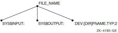
The rootnode is named FILE_NAME, and the other nodes represent the files the program uses.
3.3.3.2. File Key Domain
PCAA> PLOT/IO_SERVICES FILE_KEY BY KEYIf your program is using the secondary key more than the primary key for I/O access, you can switch key positions; primary key access is more efficient.
For RMS services that the Analyzer can plot, see Table B.1, ''RMS Services Measured by the Collector''.
3.3.3.3. File Virtual Block Number Domain
3.3.3.4. I/O System Services Domain
PCAA> PLOT/IO_SERVICES FILE_NAME BY FILEThe formal node name FILE_NAME specifies the root of a tree, and the BY clause specifies that all FILE nodes in that tree define the buckets of the histogram.
3.3.3.5. Physical Read Count Domain
PCAA> PLOT/IO_SERVICES READ_COUNT BY COUNT PCAA> PLOT/IO READ BY 10 COUNTSNote that /IO_SERVICES is the only data-kind qualifier that can be used with this domain.
3.3.3.6. Physical Write Count Domain
PCAA> PLOT/IO_SERVICES WRITE_COUNT BY COUNT PCAA> PLOT/IO WRITE BY 10 COUNTSNote that /IO_SERVICES is the only data-kind qualifier that can be used with this domain.
3.3.3.7. Total Physical I/O Count Domain
PCAA> PLOT/IO_SERVICES PHYSICAL_IO BY COUNT PCAA> TAB/IO PHYS BY 10 COUNTS
Note that /IO_SERVICES is the only data-kind qualifier that can be used with this domain.
3.3.3.8. Record Size Domain
For the record size domain, the root node is called RECORD_SIZE and the nodes represent different record sizes: zero-byte records, one-byte records, two-byte records, up to the maximum record size recorded. Figure 3.3, ''The Record Size Domain'' shows the record size tree.
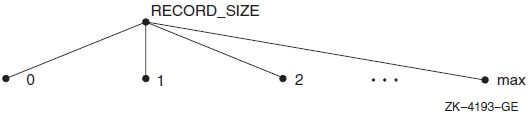
PCAA> PLOT/IO_SERVICES RECORD_SIZE BY BYTEThe resulting histogram has one bucket per record size, given in bytes. It displays the distribution of record sizes characteristic of this program's I/O, showing how many short records, long records, or in-between records the program has read or written.
PCAA> PLOT/IO_SERVICES RECORD_SIZE BY 10 BYTESIn this case, each histogram bar represents a 10-byte range of record sizes, giving a less detailed but more compact histogram.
3.3.3.9. System Services Domain
PCAA> PLOT/SERVICES SYSTEM_SERVICES BY SERVICEThis plot tells you how many times each system service is called.
Figure 3.4, ''System Services Domain'' shows how this node specification is constructed. The system services domain is represented as a tree very similar to the program tree shown in Figure 3.1, ''A Program Represented as a Tree''.
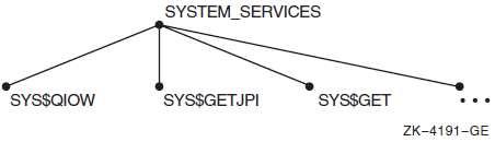
PCAA> PLOT/SERVICES SERVICE SYS$QIO, SERVICE SYS$GETJPIEach nodespec creates one bucket whose value range is defined by the corresponding system service index.
PCAA> PLOT/SERVICES/NOZEROS/DESCENDING SYSTEM_SERVICES BY SERVICEIn this case, every system service gets one histogram bar. The /NOZEROS qualifier shortens this plot by eliminating all system services that are not called. Sorting the services in descending order of use lets you examine the most-used service first.
3.3.3.10. Task Domains
|
Domain |
Node Specification |
|---|---|
|
TASK |
TASK BY TASK_IDENTIFIER |
|
TASK_IDENTIFIER task_id | |
|
TASK_TYPE |
TASK_TYPE BY TASK_TYPE_NAME |
|
TASK_TYPE_NAME task_type | |
|
TASK_PRIORITY |
TASK_PRIORITY BY n PRIORITY_UNITS |
RUN 3\%TASK 2Although this label identifies each instance of the task, it lacks a symbolic meaning. For this reason, the TASK_TYPE domain is available. The task type is the declared type of the task object. Several instances of a task may have the same type. The TASK_PRIORITY domain is the RTL priority at which each of the tasks run. The range of task priority is between 0 and 15 (this is the dynamic priority).
3.3.3.11. Time Domain
PCAA> PLOT TIME BY EVENTEach bar of the resulting histogram shows the amount of data collected after event markers for one event name in your collection run. (The Collector SETEVENT command sets event markers.) You can specify individual event names in node specifications by using the following command line.
PCAA> PLOT EVENT INPUT, EVENT COMPUTE, EVENT OUTPUTYou can also partition the time domain by millisecond ranges. For page fault, system services, task_switch, and I/O data, you can use node specifications of the form TIME BY n MSECS, where n specifies the number of milliseconds of CPU time per bucket. For example:
PCAA> PLOT/PAGE_FAULTS TIME BY 100 MSECS
You cannot specify a value of n less than 10 in a BY n MSECS clause because the CPU measures time in 10-millisecond increments.
3.3.4. Sorting the Histogram or Table
Sorting qualifiers gives you the option of displaying only buckets that are within a certain region of the histogram or table. This helps you reduce the size of the output. The sorting qualifiers specify how to sort the buckets before a histogram or table is displayed. The available sorting qualifiers are /ALPHABETICALLY, /ASCENDING, /DESCENDING, and /NOSORT.
The initial default sorting qualifier is /DESCENDING. The /NOSORT qualifier specifies no sorting at all. In that case, the Analyzer selects an order.
Sorting qualifiers are ignored for source displays. If you use the /SOURCE qualifier and a BY LINE or BY CODEPATH node specification on a PLOT or TABULATE command, the source lines are always presented in line number order regardless of the sorting qualifier.
You can specify that only the first n buckets be included in the histogram by adding =n to the sorting qualifier, or you can specify that only the buckets numbered n through m be included by adding =n:m to the sorting qualifier. The bucket numbers are assigned sequentially after sorting, and the first bucket is bucket number 1.
PCAA> PLOT/DESCENDING=20 PROGRAM BY MODULESimilarly, the following command generates a table where the buckets are first sorted alphabetically. After that, the first 10 buckets are discarded, buckets 11 through 20 are kept, and all remaining buckets are discarded:
PCAA> TABULATE/ALPHABETICALLY=11:20 PROGRAM BY MODULE
If the =n or =n:m parameters are omitted, all buckets are kept in the histogram or table.
3.3.5. Omitting Buckets of Certain Values
The bucket selection qualifiers let you remove unwanted buckets from your histogram or table. The initial default bucket selection qualifiers are /ZEROS, /NOMINIMUM, and /NOMAXIMUM.
The /NOZEROS qualifier omits buckets with a data count of zero from the histogram or table. Because buckets with a count of zero are frequently insignificant, the /NOZEROS qualifier allows you to condense a histogram or table to only those buckets that contain data. The /ZEROS qualifier retains buckets with zero data counts.
The /MINIMUM=nqualifier causes the Analyzer to omit buckets whose percentage falls below the given minimum from the histogram or table. For example, /MINIMUM=10 signifies that the Analyzer should drop all buckets whose data count is less than 10% of the total number of data points. If you use the /NOMINIMUM qualifier, no minimum threshold applies. The /NOMINIMUM and the /MINIMUM=0 qualifiers are equivalent.
Similarly, the /MAXIMUM= n qualifier deletes buckets whose percentage exceeds the given maximum from the histogram or table. The /MAXIMUM=30 qualifier omits all buckets whose data count is more than 30% of the total number of data points. If you use the /NOMAXIMUM qualifier, no maximum threshold applies. The /NOMAXIMUM and the /MAXIMUM=100 qualifiers are equivalent.
Bucket selection qualifiers are ignored for source displays. f you use the /SOURCE qualifier and a BY LINE or BY CODEPATH node specification on a PLOT or TABULATE command, the source lines are always presented in line number order regardless of the bucket selection qualifier.
3.3.6. Showing Source Code in BY LINE and BY CODEPATH Histograms and Tables
Source code display qualifiers specify whether the Analyzer displays source code next to the bars in histograms or next to the data counts in tables that are generated with BY LINE or BY CODEPATH node specifications.
The initial default source code display qualifier is /SOURCE. Use the PLOT/NOSOURCE command if you do not want to display source code in the histogram or table.
The /SOURCE qualifier has no effect if you use any node specification other than BY LINE or BY CODEPATH. When /SOURCE is in effect, the sorting qualifiers and the /NOZEROS, /MINIMUM, and /MAXIMUM qualifiers also have no effect. You always see the full source context around each source line.
3.3.7. Using CALL_TREE Node Specifications
With the PROGRAM_ADDRESS domain,you can perform specific call stack analysis by using CALL_TREE node specifications on a PLOT or TABULATE command. This results in a call tree plot that displays the call stack relationship of program units by name. As with the /STACK_DEPTH qualifier, in order to perform any kind of call stack analysis, you must first collect stack PC values in the Collector. You cannot use the /ANC, /NONCOVERAGE, /PAGE_FAULT, and /FAULT_ADDRESS qualifiers with the CALL_TREE node specification because no call stack information can be collected for them.
A call tree plot allows you to pinpoint the set of subroutine calls that is consuming most of the system's time. This is particularly useful for programs that utilize commonly-called subroutines that are known to be time-consuming. As an example, suppose your program consists of routines FILE$LOAD, FILE$UPDATE, and FILE$WRITE. The PROG BY ROUTINE nodespec may create a plot that shows most of your time being spent in FILE$WRITE. However, the CALL_TREEBY CHAIN_ROUTINE nodespec may show that most of the time was spent performing the FILE$WRITE routine when called from the FILE$LOAD routine.
Each bucket in the plot is a call chain. A call chain is the set of return addresses found on the call stack associated with each data point. The Analyzer attempts to match each PC value on the call stack to a program unit. Any PC value that cannot be matched to a program address unit is resolved to a "best guess," such as a shareable image or the hexadecimal representation.
The Analyzer creates the call tree plot by scanning the data file once to determine all the measured call chains, then again to match the data points to the specified buckets. The set of measured call chains is the domain. The CALL_TREE node specification represents that domain.
CALL_TREE BY CHAIN_MODULE
CALL_TREE BY CHAIN_ROUTINE
CALL_TREE BY CHAIN_LINE
CHAIN_MODULE chain_name
CHAIN_ROUTINE chain_name
CHAIN_LINE chain_name
Note
For case-sensitive languages, use the SET LANGUAGE command to permit the correct parsing. For example, to handle C identifiers and FORTRAN identifiers in the same call chain, set the language to C and use uppercase for all the FORTRAN identifiers.
PCAA> PLOT/NOCHAIN_NAME CALL_TREE BY CHAIN_ROUTINE
Performance and Coverage Analyzer Page 1
Program Counter Sampling Data (1156 data points total) - "*"
Percent Count Call Chain Name
1.2% Chain : MAIN_PROGRAM
5.5% ** Chain : . ROUTINE_A
6.5% ** Chain : . . UTILITY_ROUTINE_A
12.5% ***** Chain : . ROUTINE_B
3.5% * Chain : . ROUTINE_C
1.4% Chain : . . SHARE$FORRTL
15.5% ******* Chain : . . UTILITY_ROUTINE_A
2.3% * Chain : . . ROUTINE_D
0.4% Chain : . . ROUTINE_EIn Example 3.7, ''Indented Call Tree Plot'', a routine name is indented by two characters if that routine was called by another routine. The call levels are hierarchical. That is, MAIN_PROGRAM called ROUTINE_A, ROUTINE_B, and ROUTINE_C directly. ROUTINE_A in turn called UTILITY_ROUTINE_A. ROUTINE_B did not call any other routines, and so on.
The counts and percentages shown are those that occurred in the routines. The /CUMULATIVE qualifier can be used to find the data counts in a given routine, plus all of its calls. The /MAIN_IMAGE and /STACK_DEPTH qualifiers will start the call chains that begin at the specified point on the call stack. The /ALPHABETICALLY[=[n:]m] qualifier provides an alphabetical sort on the first 255 characters of each call chain in a call tree plot.
If you specify /NOCHAIN_NAME, then the PLOT command's maximum,minimum, and sorting qualifiers are ignored. If you specify /CHAIN_NAME, then these qualifiers are in effect.
PCAA> PLOT/CHAIN_NAME CALL_TREE BY CHAIN ROUTINE
Performance and Coverage Analyzer Page 1
Program Counter Sampling Data (1156 data points total) - "*"
Percent Count Call Chain Name
1.2% Chain : MAIN_PROGRAM
5.5% ** Chain : MAIN_PROGRAM,ROUTINE_A
6.5% ** Chain : MAIN_PROGRAM,ROUTINE_A,
UTILITY_ROUTINE_A
12.5% ***** Chain : MAIN_PROGRAM,ROUTINE_B
3.5% * Chain : MAIN_PROGRAM,ROUTINE_C
1.4% Chain : MAIN_PROGRAM,ROUTINE_C,
UTILITY_ROUTINE_A
15.5% ******* Chain : MAIN_PROGRAM,ROUTINE_C,SHARE$FORRTL
2.3% * Chain : MAIN_PROGRAM,ROUTINE_C,ROUTINE_D
0.4% Chain : MAIN_PROGRAM,ROUTINE_C,ROUTINE_EThe comma list form of a call tree plot is useful when specifying sorting options.
3.3.8. Specifying Which Program Counter Values to Tally
Program address selection qualifiers determine which program addresses the Analyzer selects before tallying them in a histogram or table. The initial default program address selection qualifiers are /NOSTACK_DEPTH and /NOCUMULATIVE.
The /[NO]MAIN_IMAGE default depends on the data kind being plotted. If stack PCs have been collected, then /MAIN_IMAGE is the default. In all other cases, /NOMAIN_IMAGE is the default. For example, SETPC_SAMPLING in the Collector defaults to collecting stack PCs, and therefore /MAIN_IMAGE is the default in the Analyzer's PLOT command. SET COUNTERS does not default to collecting stack PCs, and therefore the Analyzer uses /NOMAIN_IMAGE as the default.
3.3.8.1. Performing Call Stack Analysis
To perform any kind of call stack analysis, you must first collect stack PC values in the Collector. The /MAIN_IMAGE[=prog-unit], /STACK_DEPTH=n, and /CUMULATIVE[=n] qualifiers use call stack return addresses (stack PC values) when creating histograms and tables.
The /MAIN_IMAGE qualifier causes the Analyzer to tally the first program address on the call stack that falls within the program's address range. (This value may be the original PC value.) If much of your data falls in shareable images, use the /MAIN_IMAGE qualifier to instruct the Analyzer to charge back that data to the places in your program (the main image) that call the shareable images.
The /NOMAIN_IMAGE qualifier causes the Analyzer to use the original PC value for each data point.
3.3.8.2. Defining the Program Unit as the Main Image
You can define the main image by specifying a program unit with the /MAIN_IMAGE=prog-unit qualifier. By default, the program unit is the entire user program but it can be a module, routine, or line. Specifying the program unit you want starts the call stack at that point. If no program address on the stack is within the program unit's address range, then it does not appear in any of the buckets and is added to the total of "Data points failing /STACK_DEPTH or /MAIN_IMAGE" that appears on the summary page.
Note that the SYSTEM$SERVICE and the SYSTEM$SPACE program units that represent the system service vector and the system space can be used in the /MAIN_IMAGE=prog-unit qualifier.
3.3.8.3. Performing Specific Call Stack Analysis
You can accomplish more specific call stack analysis with the /STACK_DEPTH qualifier. With the /STACK_DEPTH=n qualifier, the Analyzer selects data points that are n call frames lower than the return address you specified with the /MAIN_IMAGE qualifier. You must specify an integer that is greater than or equal to one. Each increment in the integer represents going one more call frame lower in the stack. The /STACK_DEPTH=1 qualifier causes the address of the caller to be charged, /STACK_DEPTH=2 causes the address of the caller's caller to be charged, and so on. If you specify a number that is greater than the number of call frames on the stack, then the corresponding program address will not appear in any of the buckets; rather, it will be added to the summary total of "Data points failing /STACK_DEPTH or /MAIN_IMAGE" that appears on the summary page.
The /NOSTACK_DEPTH qualifier, the initial default, specifies that no stack depth analysis be performed and causes the original PC to be used.
3.3.8.4. Tallying Program Counter Values
The /CUMULATIVE qualifier determines whether all program counter values on the call stack are tallied or if only one is tallied. The /CUMULATIVE qualifier causes the Analyzer to tally all stack PC values. You can use the/CUMULATIVE=n qualifier to request that only n return addresses down the stack be tallied. Thereby, the Analyzer adds each data point in many buckets of the histogram or table. The effect is that each bucket shows how much time or other resource is consumed not only by the corresponding program unit but also by all return addresses (or n return addresses if /CUMULATIVE=n that call that unit directly or indirectly).
For example, if you plot program counter sampling data by routine for the whole program, using the /CUMULATIVE qualifier, then each data point is tallied in the buckets for the routine in which it was collected, for the caller of that routine, for the caller of the caller, and so on (or for the number of calls specified with /CUMULATIVE=n). All data points are tallied in the bucket for the main routine because the main routine is always the ultimate caller; the main routine contains 100% of the data points. The histogram bar for each routine shows how much time is consumed in that routine and in all routines it calls.
The /NOCUMULATIVE qualifier causes only the first program counter value to be tallied; other stack PC values are not used.
3.3.8.5. Using Program Address Selection Qualifiers
If you use all the program address selection qualifiers together, they are applied in the following order: /MAIN_IMAGE, /STACK_DEPTH, then /CUMULATIVE. Therefore, if you specify the /MAIN_IMAGE=prog-unit and /STACK_DEPTH=nqualifiers, the Analyzer searches the stack for the first address within the specified program unit. However, it does not charge the data point to this address, but to the address n call frames on the stack from the main image address. If you include /CUMULATIVE on that command, the same action occurs, but the Analyzer also charges the data point to every caller (or n callers if /CUMULATIVE=n) below the address that was charged.
PCAA> TABULATE/MAIN=ROUTINE_1/STACK=1/CUM PROG BY ROUTINENote the acceptable abbreviated forms of /STACK_DEPTH, /MAIN_IMAGE, and /CUMULATIVE that are used.
3.3.9. Filling and Scaling the Histogram
Design qualifiers let you determine the character fill to be used for the histogram bar, to adjust the scale of the histogram, and to wrap plot output that is too long. Each of these features is useful in controlling the appearance of the plot. The design qualifiers are /FILL, /SCALE, /[NO]WRAP, /[NO]KEEP, and /[NO]TREE. The /FILL and /SCALE qualifiers are described in the following sections. See the VSI DECset for OpenVMS Performance and Coverage Analyzer Reference Manual for more information on them, as well as complete descriptions for the /[NO]WRAP, /[NO]KEEP, and /[NO]TREE qualifiers.
3.3.9.1. Defining the Character String for the Histogram Bar
Use the /FILL qualifier to define the character string that makes up the histogram bar. This is useful when building a multiple data-kind plot. /FILL= "a", where "a" is a character string delimited by double or single quotation marks, specifies a fill of character string "a" for the data kind in the first position in the plot. /FILL=("a", "b", …) specifies a fill of character string "a" for the first data kind, a fill of character string "b" for the second data kind, and so on. A series of character string specifications are enclosed within parentheses. A maximum of eight character strings can be defined. Note that blanks, spaces, and other nonprinting ASCII characters should not be used in this string because it will be used as the fill in a plot. The standard default fill for each of the eight positions is listed in the online PCA Command Dictionary under the PLOT command.
3.3.9.2. Setting the Range for the Histogram Bar
By default, histogram scales are adjusted so that the longest bar occupies the full width of the plot. This adjusted scale is convenient for viewing individual histograms, but can make comparing histograms with each other difficult. When comparing histograms, you can set the range of the histogram bar with the /SCALE=nqualifier on the PLOT, TABULATE, and SET PLOT commands. /SCALE=n selects a fixed scale, set to n percent, where n is an integer value from 1 to 100. To restore the default scale, specify the /NOSCALE qualifier on the PLOT, TABULATE, or SET PLOT command.
PCAA> PLOT/SCALE=75This command will cause the longest bar to occupy about half of the histogram width.
Fixed scaling can cause histogram bars to represent percentages that are larger than the histogram range. In plots produced with /NOSOURCE, these bars are truncated to equal the specified range, and the right-angle character (>) appears in the rightmost position of the bar. In plots produced with /SOURCE, the left-angle character (<)appears in the leftmost position of the truncated bar.
The fixed scaling option can be useful when comparing multiple data kinds in one histogram. In multiple data-kind plots, the scaling option used for the first data kind also applies to subsequent data kinds included in the plot.
3.3.10. Performing Multi-tasking Analysis
You can gather tasking information with the SET TASKING Collector command,and then in the Analyzer use task qualifiers to perform multi-tasking analysis.
The /TASK_SWITCH qualifier selects a data kind that represents the number of times there was a task context switch. It can be applied to the following domains: TIME BY n MSECs, TASK, TASK_PRIORITY, and TASK_TYPE. This qualifier will only work with the TIME, TASK, TASK_PRIORITY, and TASK_TYPE filter specifications.
The /CREATOR_PC qualifier selects a program address that charges a data point to the location in the program that created the task, rather than to the PC value of the measurement. This qualifier can only be used when the PROGRAM_ADDRESS domain is in effect, and when tasking data has been collected. It overrides /MAIN_IMAGE, /STACK_DEPTH, and /CUMULATIVE.
The /PARENT_TASK qualifier charges a data point to the parent of the current task, rather than to the current task. It can only be used when the TASK or the TASK_TYPE domain is in effect, and when tasking data has been collected.
3.3.11. Interpreting TABULATE Confidence Intervals
PCAA> TABULATE/PC PROGRAM BY ROUTINE
Performance and Coverage Analyzer Page 1
Program Counter Sampling Data (386 data points total)
Data 95% Conf
Bucket Name Count Percent Interval
PROGRAM_ADDRESS\
PRIMES . . . . . . . . . . 3 0.8%
PRIME . . . . . . . . . . 239 61.9% +/- 4.8%
READ_RANGE . . . . . . . . 18 4.7% +/- 2.1%
READ_END_OF_FILE . . . . . 0 0.0%
READ_ERROR . . . . . . . . 0 0.0%
OUTPUT_TO_DATAFILE . . . . 1 0.3%
SHARE$FORRTL . . . . . . . 21 5.4% +/- 2.3%
SHARE$LIBRTL . . . . . . . 10 2.6% +/- 1.6%
SHARE$PCA$COLLECTOR . . . 0 0.0%
SHARE$DBGSSISHR . . . . . 0 0.0%
SHARE$PCA$PRVSHR . . . . . 0 0.0%
SHARE$LBRSHR . . . . . . . 0 0.0%
SHARE$SMGSHR . . . . . . . 0 0.0%
PCAA>The Analyzer computes the percentage of PC values that fall in each bucket by dividing the data count on the same line by the total number of PC values collected (the sample size) and multiplying by 100. This yields the percentage of the total execution time consumed in the corresponding routine or other program unit.
However, these measurements are random sampling processes. This means that the number of PC values collected in a given routine may not be exactly proportional to the amount of time consumed in that routine. Random variations in the sampling process may cause more PC values to be collected from one routine than from another, even if the two routines take exactly the same amount of time. Unpredictable variations in system load, interrupt processing, and disk access times are among the causes of random variation in the PC sampling process.
Obtaining the true percentage of time spent in each routine (or whatever program units you are tabulating) based on PC sampling data is impossible. The computed percentage is only an estimate of the true percentage. However, using this estimated percentage and the sample size, you can compute a confidence interval for the true percentage. To help understand how close the estimate is likely to be to the true percentage, the Analyzer computes a 95%confidence interval around the estimated percentage, assuming a normal distribution.
The interpretation of the confidence interval is as follows. If the computed percentage (the estimate) is 13.0% and the 95% confidence interval is expressed as +/– 2.0%, then the confidence interval is 11% to 15%.This means you can be 95% confident that the true percentage is in this range.
If the data count is within 3 of zero or within 3 of the total sample size, noconfidence interval is computed. For such small deviations from 0% or from 100%, the formula used to compute the confidence interval may not be statistically valid. Therefore, the confidence interval is left blank in the TABULATE output.
3.4. Creating a Multiple Data-Kind Plot
You can compare more than one data kind in the same plot. For example, you can plot PC sampling hits, page fault addresses, and I/O service calls in the same histogram to determine if the PC sampling spikes are caused by page faults or by I/O service calls.
PCAA> PLOT/PC_SAMPLING/FILL=("pc") PROGRAM BY ROUTINE
Performance and Coverage Analyzer Page 1
Program Counter Sampling Data (11236 data points total) - "pc"
Bucket Name +----+----+----+----+----+----+----+----+----+----+
SYSTEM$SERVICE\ |
SYSTEM$SERVICE.|pcpcpcpcpcpcpcpcpcpcpcpcpcpcpcpcpcpcpcpcpcpcpcpcpc 40.2%
SYSTEM$SPACE\ |
SYSTEM$SPACE . |pcpcpcpcpc 7.9%
BUCKETS\ |
BUCKETS . . . |pc 1.4%
AVERAGES\ |
AVERAGES . . . | 0.2%
CODLNS\ |
CODLNS . . . . | 0.2%
MATCHREC\ |
MATCHREC . . . | 0.1%
MATCHST1\ |
MATCHST1 . . . | 0.0%
|
|
|
+----+----+----+----+----+----+----+----+----+----+
Performance and Coverage Analyzer Page 1PCAA> INCLUDE/IO_SERVICES/MAIN_IMAGE
Performance and Coverage Analyzer Page 1
Program Counter Sampling Data (138 data points total) - "pc"
I/O System Service Calls (108 data points total) - "io"
Bucket Name ----+----+----+----+----+----+----+----+----+----+
PRIMES\ |
WRITELN . . . |pcpcpcpcpcpcpcpcpcpcpcpcpcpcpcpcpcpcpcpcpcpcpc 87.7%
|ioioioioioioioioioioioioioioioioioioioioioioio 94.4%
OPENIN . . . . |pc 4.3%
|i 1.9%
PUTINT . . . . |pc 2.9%
| 0.0%
LISTPRIMES . . |p 2.2%
| 0.0%
CLOSEIN . . . | 0.7%
| 0.9%
OPENOUT . . . | 0.7%
|i 1.9%
PRIME . . . . | 0.7%
| 0.0%
PUTSTR . . . . | 0.7%
| 0.0%
CLOSET . . . . | 0.0%
| 0.9%
READING . . . | 0.0%
| 0.0%
READLN . . . . | 0.0%
| 0.0%
SYSTEM$SERVICE\ |
SYSTEM$SERVICE | 0.0%
| 0.0%
SYSTEM$SPACE\ |
SYSTEM$SPACE . | 0.0%
| 0.0%
+----+----+----+----+----+----+----+----+----+----+
PCAA> INCLUDE/PAGE_FAULTS/FILL="pf"
Performance and Coverage Analyzer Page 1
Program Counter Sampling Data (11236 data points total) - "pc"
I/O System Service Calls (3581 data points total) - "io"
Page Fault Program-Counter Data (121 data points total) - "pf"
Bucket Name ----+----+----+----+----+----+----+----+----+----+
SYSTEM$SERVICE\ |
SYSTEM$SERVICE |pcpcpcpcpcpcpcpcpcpcpcpcpcpcpcpcpcpcpcpcpcpcpcpc 40.2%
| 0.0%
| 0.0%
SYSTEM$SPACE\ |
SYSTEM$SPACE . |pcpcpcpcpc 7.9%
| 0.0%
|pfpfpfpfpfpfpfpfpfpfpfpfpf 19.8%
BUCKETS\ |
BUCKETS . . . |pc 1.4%
|ioioioioioioioioioioioioioioioioioioioioioioioio 97.7%
|pfpfpfpfpfpfpfpfpfpfpfpfpfpfpfpfpfpfpfpfpfpfpfpf 38.0%
|
|
|
+----+----+----+----+----+----+----+----+----+----+PCAA> INCLUDE/MAIN_IMAGE
Performance and Coverage Analyzer Page 1
Program Counter Sampling Data (11236 data points total) - "pc"
I/O System Service Calls (3581 data points total) - "io"
Page Fault Program-Counter Data (121 data points total) - "pf"
Program Counter Sampling Data (11236 data points total) - "@"
Bucket Name ----+----+----+----+----+----+----+----+----+----+
SYSTEM$SERVICE\ |
SYSTEM$SERVICE.|pcpcpcpcpcpcpcpcpcpcpcpcpcpcpcpcpcpcpcpcpcpcpcpcpc 40.2%
| 0.0%
| 0.0%
| 0.0%
SYSTEM$SPACE\ |
SYSTEM$SPACE . |pcpcpcpcpc 7.9%
| 0.0%
|pfpfpfpfpfpfpfpfpfpfpfpfpf 19.8%
| 0.0%
|
|
|
|
+----+----+----+----+----+----+----+----+----+----+The INCLUDE command uses a subset of PLOT qualifiers and parameters. See the online PCA Command Dictionary for a listing of qualifiers and parameters for the INCLUDE command. The default qualifiers are taken from the currently active plot.
There is a maximum of eight data kinds per plot.
The data kinds must be compatible with the node specifications for the current plot.
There is an active plot available.
A different filter or restriction can be applied to the data kind for every INCLUDE command, by entering SET FILTER commands between the INCLUDE commands. The current filters are applied to all data kinds when the INCLUDE command is entered. The newly created plot will appear after you enter the INCLUDE command.
PCAA> EXCLUDE
Performance and Coverage Analyzer Page 1
Program Counter Sampling Data (11236 data points total) - "pc"
I/O System Service Calls (3581 data points total) - "io"
Page Fault Program-Counter Data (121 data points total) - "pf"
Bucket Name +----+----+----+----+----+----+----+----+----+----+
SYSTEM$SERVICE\ |
SYSTEM$SERVICE.|pcpcpcpcpcpcpcpcpcpcpcpcpcpcpcpcpcpcpcpcpcpcpcpcpc 40.2%
| 0.0%
| 0.0%
SYSTEM$SPACE\ |
SYSTEM$SPACE . |pcpcpcpcpc 7.9%
| 0.0%
|pfpfpfpfpfpfpfpfpfpfpfpfpf 19.8%
BUCKETS\ |
BUCKETS . . . |pc 1.4%
|ioioioioioioioioioioioioioioioioioioioioioioioioio 97.7%
|pfpfpfpfpfpfpfpfpfpfpfpfpfpfpfpfpfpfpfpfpfpfpfpfpf 38.0%
|
|
|
+----+----+----+----+----+----+----+----+----+----+When you switch data files, any information that depends on the symbol table in the current data file is lost. This information includes the currently active plot, the current default node specifications, and any filters you may have set.
3.4.1. Merging PCA Performance and Software Performance Monitor (SPM) Files
Merge data from one or more performance data files into another performance data file, where all the files have been created in succession for the same image. While this may sometimes be convenient, it is usually simpler and more efficient to use the SET DATAFILE/APPEND command in the Collector.
Merge data from one or more SPM data files into a performance data file. This is the only way to make SPM data available for analysis with PCA. You must ensure that the merged SPM data pertains to the image for which the output performance data file has been created. This is because PCA cannot perform all the necessary checks for SPM data.
Merge ANC information from an old performance data file to a newer one that was created for the same program. Note that all coverage set information (no tjust ANC information) is merged for each unchanged routine. This preserves the proper context for the ANC information.
Merge data from one or more performance data files into another performance data file, where all the files have been created simultaneously for the same image, and have been executed in a parallel processing environment. Note that the MERGE operation preserves collection run names. After all the data has been merged, you can use the original collection run names to analyze any subset of the parallel collections. Thereby, important insight can be gained into the performance of the parallel processing itself, in addition to the performance of the image being run.
$ PERFORMANCE[/INTERVAL=ticks] [/IDENTIFICATION=process-id]- _$ COLLECT=SYSTEM_PCPC values are then sampled at a specified interval. You can specify the interval in the range of 1 to 100 ticks with the /INTERVAL qualifier, where each tick equals 10 milliseconds. The resulting PC log file includes the PC values for all processes on the system, unless you select a single process with the /IDENTIFICATION qualifier. The MERGE command accepts SPM data only from system-wide PC log files, hereafter referred to as SPM data files.
Data merged from SPM data files must have been gathered for the same image as the image for the currently open performance data file. To prepare the image for data collection with SPM and with the Collector, you may link the image with the /DEBUG qualifier. Then, to collect data with SPM, run the image with /NODEBUG.
3.5. Listing the Raw Performance Data
To view the raw data gathered by the Collector, use the LIST command to display a list of the raw performance data.
Enter the FILE command.
Use the PRINT command to print the output.
PCAA> LIST ALL
PCAA> LIST SERVICES, IO_SERVICES, PAGE_FAULTS
To see a complete list of the LIST qualifiers, refer to the LIST command in the Command Dictionary section of the VSI DECset for OpenVMS Performance and Coverage Analyzer Reference Manual.
PCAA> SHOW RUN_DESCRIPTION 2:4
PCAA> LIST/START_TIME
The parameter default is NOSTART_TIME.
You can specify a run name as the parameter. If you use the SET RUN_NAME EVENT1 command in the Collector, you can use the SHOW RUN_DESCRIPTION EVENT1 in the Analyzer.
PCAA> SHOW RUN_DESCRIPTION *
3.6. Using Acceptable Noncoverage (ANC)
Most programs have portions of code that you would not expect to be tested; for example, internal error paths, difficult-to-test paths, and so on. These portions of code are considered acceptably noncovered, or ANC.
Once you have decided which portions of a program are acceptably noncovered, you can save that information for the next test run.
If you have modified the program and you want to preserve the ANC information from a previous version of the program, then you can use the MERGE/ANC command to copy the ANC information from the old data file to the new one. The information will only be copied for those routines in the program that have not changed. PCA decides if a routine has changed by looking at two sets of codepath information for each routine. One set is from the current version of the program, and the other (saved) set is from a previous version. If the codepath information has not changed, then the ANC information is considered valid, and is merged. If the codepath information has changed, then the ANC information is disregarded by MERGE/ANC for the given routine. See the online PCA Command Dictionary for complete information about the MERGE command.
There are two ways to specify ANC information. One is to generate a noncoverage plot or tabulation, then use a traverse command (such as NEXT) or the FIND command to pinpoint a particular noncovered point. Then, enter the SET ANC command at the Analyzer prompt. The SET ANC command declares all the noncovered points within the selected bucket's address range as acceptably noncovered. If you use the SET ANC command in this manner when the FIND pointer is pointing to a routine bucket, then all the lines or codepaths within the routine are flagged as ANC, whether they are covered or not. You can continue traversing the plot in this manner until you have reviewed all the noncovered points. Use the NEXT command to move the pointer from one noncovered point to another.
PCAA> SET ANC ROUTINE R2 BY LINE, ROUTINE R4 BY LINEThe nodespec must specify one or more program address locations.
ANC information is stored in the coverage-set table section in the performance data file. You can list the full contents of that table with the LIST/COVERAGE_SET command. The SHOW ANC command displays the current status of ANC information.
If you want to remove ANC information from the coverage-set table, use the CANCEL ANC command. If you enter the CANCEL ANC command without a nodespec, then it pertains to all the ANC points within the bucket pointed to with a FIND or traverse arrow. You can provide a nodespec on this command to specify which ANC points to remove. You can also use the CANCEL ANC/ALL command to remove all the ANC information from the current data file.
PCAA> SET FILTER F1 PROGRAM_ADDRESS=%ANCSee the online PCA Command Dictionary for complete information on the SET FILTER command.
Section 4.5, ''Determining Acceptable Noncoverage (ANC)'' contains an example of the complete cycle of merging, setting, and using ANC information.
3.7. Editing Source Code from Within the Analyzer
If you want to edit the source code displayed by the most recent PLOT or TABULATE command, you can use the EDIT command to invoke an editor directly from the Analyzer. The Language-Sensitive Editor (LSE) is the default editor. To use the EDIT command,you must have an editor installed on your system. For more information on LSE, see the Guide to VSI Language-Sensitive Editor for OpenVMS Systems.
The editor you select must be one you can access from DCL level. Use the Analyzer SET EDITOR command to specify the editor you want to use. This will cause subsequent EDIT commands to invoke the editor you chose.
The SET EDITOR command accepts the following qualifiers: /CALLABLE_EDT, /CALLABLE_LSEDIT, /CALLABLE_TECO, and /CALLABLE_TPU.
PCAA> SET EDITOR/CALLABLE_TPU
PCAA> SHOW EDITOR
The editor is CALLABLE_TPU having the command line:
"TPU"You
can specify a command line if you use the /CALLABLE_LSEDIT or the /CALLABLE_TPU
qualifiers, but not if you use the /CALLABLE_EDT or the /CALLABLE_TECO
qualifiers.PCAA> EDITThis command spawns a subprocess to run the editor. The Analyzer automatically positions the editor at the point in the source file displayed by the PLOT or TABULATE command. When you exit from the editor, the Analyzer session resumes.
If you use the /EXIT qualifier on the EDIT command, you terminate the Analyzer session and invoke the editor in the same process.
PCAA> EDIT MODNAME\25If you omit the module name and backslash, the editor defaults to the module referenced by the PLOT or TABULATE command currently in effect.
PCAA> SET EDITOR/CALLABLE_LSEDIT/START_POS "LSED/READ_ONLY"
Also, the /START_POSITION qualifier will be appended to the command line, causing the editing session to start on the source line that the Analyzer is currently pointing to. Note the abbreviated form of /START_POSITION. Also note that the command line is enclosed in quotation marks.
3.8. Using Initialization Files and Command Procedures
The Analyzer initialization file is automatically read and executed at the start of each session. It is useful for defining frequently used keypad keys or command abbreviations, establishing mode settings, such as screen mode or SET PLOT defaults, or setting up a SET SOURCE command.
$ DEFINE PCAA$INIT ANL_STARTUP.PCAA
After reading the initialization file, the Analyzer solicits additional command input from the terminal until you enter the EXIT command.
To make command entry more efficient, you can place often-used commands into a command procedure. For example, you can use command procedures for lengthy but frequently used filter specifications.
Analyzer command procedures are similar to Collector command procedures discussed in Section 2.8, ''Using Collector Command Procedures''.
3.8.1. Using Analyzer Logical Names
PCAA$INIT
PCAA$INPUT
PCAA$OUTPUT
SYS$LP_LINES
SYS$PRINT
PCAA$DECW$DISPLAY
Table B.5, ''Analyzer Logical Names'' describes the logical names the Analyzer accepts.
Chapter 4. Productivity Enhancements with PCA
The examples in this chapter demonstrate how to use PCA to solve common problems and improve the performance of your applications. Section 4.7, ''Using PCA in Screen Mode'' shows how to use the Analyzer in screen mode.
Section 4.1, ''Example 1: Reducing Execution Time'' demonstrates how to find where most of the time is being spent in a typical application, then applies a change that improves that program's performance.
Section 4.2, ''Example 2: Analyzing Call Stack Data'' demonstrates the analysis of call stack data.
Section 4.3, ''Example 3: Using Multiple Data Kinds'' demonstrates how a multiple data-kind plot can isolate the reason a program statement takes the most time.
Section 4.4, ''Example 4: Using Event Markers for Selective Analysis'' demonstrates the use of event markers for selective analysis.
Section 4.5, ''Determining Acceptable Noncoverage (ANC)'' demonstrates the collection and analysis of coverage data,and shows how you can determine acceptable noncoverage.
Section 4.6, ''Example 6: Measuring Ada Tasking Data'' demonstrates the measurement of Ada tasks.
Some of the programs used in this chapter are compiled with the /NOOPTIMIZE qualifier because they are so simple the compiler would otherwise optimize away the effect that the examples are intended to show.
4.1. Example 1: Reducing Execution Time
This example demonstrates a simple method of finding out where most of the time is being spent in a typical application.
PCA is used on a FORTRAN program that counts the prime numbers within a given range. The Collector gathers PC sampling data. Then the Analyzer is invoked specifying the performance data file PCA$PRIMES. When you enter the NEXT command, the Analyzer creates a source plot, pointing to the most significant line.
$ FOR/NOOPTIMIZE/DEBUG PCA$PRIMES.FOR
$ LINK/DEBUG PCA$PRIMES
$ DEFINE LIB$DEBUG PCA$COLLECTOR.EXE
$ RUN PCA$PRIMES
PCA Collector Version 5.0
PCAC> GO
%PCA-I-DEFDATFIL, set datafile required in this context, creating
'[]PCA$PRIMES.PCA'
%PCA-I-BEGINCOL, data collection begins
%PCA-I-DATADEFPC, defaulting to collecting PC sampling data
169 prime numbers generated between 1 and 1000
FORTRAN STOP
%PCA-I-ENDCOL, data collection ends
$ PCA PCA$PRIMES

         Performance and Coverage Analyzer Version 5.0

PCAA> NEXT Performance and Coverage Analyzer Page 1
Program Counter Sampling Data (93 data points total) - "*"
Routine PRIME\PRIME
Percent Count Line
PRIME\PRIME\
0.0% 5: LOGICAL FUNCTION PRIME(NUMBER)
0.0% 6: PRIME = .TRUE.
0.0% 7: DO 10 I = 2, NUMBER/2
33.3% ******* -> 8: IF ((NUMBER - ((NUMBER / I) * I)) .EQ.
0) THE
-: N
0.0% 9: PRIME = .FALSE.
0.0% 10: RETURN
11: ENDIF
2.2% 12: 10 CONTINUE
0.0% 13: RETURN
The resulting source plot shows that 33.3% of the time is spent at line 8. This is expected,because this is where the calculation that determines the prime is done. To reduce the time spent at line 8, you must either make the calculation more efficient or reduce the number of times the calculation is done. At this point, confirm that the time being spent is caused by CPU consumption.
Gathering and Analyzing CPU Sampling Data
$ RUN PCA$PRIMES

        PCA Collector Version V5.0

PCAC> SET DATAFILE/APPEND/EXE
PCAC> SET CPU_SAMPLING
%PCA-I-PCDISTORT, PC sampling data may be distorted by collection of other data
%PCA-I-CPUDISTOR, CPU sampling data may be distorted by collection of other data
PCAC> GO
%PCA-I-BEGINCOL, data collection begins
 169 prime numbers generated between    1 and 1000
FORTRAN STOP
%PCA-I-ENDCOL, data collection ends

$$ PCA PCA$PRIMES
Performance and Coverage Analyzer Version V5.0
PCAA> PLOT/CPU Performance and Coverage Analyzer Page 1
CPU Sampling Data (114 data points total) - "*"
Bucket Name +----+----+----+----+----+----+----+----+
PRIME\ |
PRIME . . . . . . |***************************************** 62.3%
OUTPUT_TO_DATAFILE\ |
OUTPUT_TO_DATAFILE |*************** 19.3%
READ_RANGE\ |
READ_RANGE . . . . |******** 10.5%
PCA$PRIMES\ |
PCA$PRIMES . . . . |****** 7.9%
READ_END_OF_FILE\ |
READ_END_OF_FILE . | 0.0%
READ_ERROR\ |
READ_ERROR . . . . | 0.0%
SYSTEM$SERVICE\ |
SYSTEM$SERVICE . . | 0.0%
SYSTEM$SPACE\ |
SYSTEM$SPACE . . . | 0.0%
|
|
+----+----+----+----+----+----+----+----+PCAA> CTRL/N
                    Performance and Coverage Analyzer                Page 1
                CPU Sampling Data (114 data points total) - "*"
                              Routine PRIME\PRIME
Percent   Count       Line
PRIME\PRIME\
  0.0%                   5:         LOGICAL FUNCTION PRIME(NUMBER)
  0.0%                   6:         PRIME = .TRUE.
  0.0%                   7:         DO 10 I = 2, NUMBER/2
 58.8%  ******* ->       8:         IF ((NUMBER - ((NUMBER / I) * I)) .EQ.
                                                                   0) THE
                         -: N
  0.0%                   9:             PRIME = .FALSE.
  0.0%                  10:             RETURN
                        11:         ENDIF
  3.5%                  12:    10   CONTINUE
  0.0%                  13:         RETURN
This confirms that CPU consumption, caused by a CPU-intensive instruction, is the problem.
Editing and Modifying the Program
PCAA> EDIT
$ FOR/NOOPT/DEBUG PCA$PRIMES.FOR
$ LINK/DEBUG PCA$PRIMES
$ DEFINE LIB$DEBUG PCA$COLLECTOR.EXE
$ RUN PCA$PRIMES

        PCA Collector Version V5.0

PCAC> GO
%PCA-I-DEFDATFIL, set datafile required in this context, creating
'[]PCA$PRIMES.PCA'
%PCA-I-BEGINCOL, data collection begins
%PCA-I-DATADEFPC, defaulting to collecting PC sampling data
1000 prime numbers generated between     1 and 1000
FORTRAN STOP
%PCA-I-ENDCOL, data collection ends
$ PCA PCA$PRIMES
Performance and Coverage Analyzer Version V5.0
PCAA> CTRL/N Performance and Coverage Analyzer Page 1
Program Counter Sampling Data (90 data points total) - "*"
Percent Count Line
PRIME\
1: C Function to identify whether the number in
2: C in the given range is prime number or not.
3: C If so, returned function value is TRUE.
4: C
3.3% * 5: LOGICAL FUNCTION PRIME(NUMBER)
6: C
7: REAL*8 R
0.0% 8: PRIME = .TRUE.
0.0% 9: R = NUMBER
4.4% * 10: DO 10 I = 2, (SQRT(R))
11: C
46.7% ******** 12: IF ((NUMBER - ((NUMBER / I) *
I)) .EQ. 0) THEN
1.1% 13: PRIME = .FALSE.
0.0% 14: RETURN
15: ENDIF
16: C
6.7% * 17: 10 END DO
18: C
0.0% 19: RETURN
20: ENDThe percentage of time spent at the calculation is smaller now, but some of the other percentages are larger. The modification has reduced the relative time spent at one line, causing the same amount of time at another line to be a larger portion of the total time.
Relative measures do not always confirm that performance has been improved. Actual timing of the execution is used to confirm that a program performs better (particularly if the changes are extensive). Sometimes, changes only move a "bottleneck" to another place in the program.
4.2. Example 2: Analyzing Call Stack Data
In this example, the Collector gathers PC sampling data and I/O services data on the Pascal program PCA$8QUEENS. Both data kinds are gathered with calls tack return addresses. Then, the data is analyzed to find out what portions of the program are causing the I/O calls. This example runs optimized code so you can go directly to the real "hot spots", avoiding sections of code that can be optimized by the compiler.
$ PASCAL/DEBUG PCA$8QUEENS.PAS
$ LINK/DEBUG PCA$8QUEENS
$ DEFINE LIB$DEBUG PCA$COLLECTOR.EXE
$ RUN PCA$8QUEENS

        PCA Collector Version V5.0

PCAC> SET PC_SAMPLING/STACK_PCS
PCAC> GO
%PCA-I-DEFDATFIL, set datafile required in this context, creating
'[]PCA$PCA$8QUEENS.PCA'
%PCA-I-BEGINCOL, data collection begins
%PCA-I-ENDCOL, data collection ends

$ RUN PCA$8QUEENS

        PCA Collector Version V5.0

PCAC> SET IO_SERVICES/STACK_PCS
PCAC> GO
%PCA-I-DEFDATFIL, set datafile required in this context, creating
'[]PCA$PCA$8QUEENS.PCA'
%PCA-I-BEGINCOL, data collection begins
%PCA-I-ENDCOL, data collection ends

$
The /STACK_PCS qualifier, although used in this example, is the default setting for both kinds of data being gathered.
$ PCA PCA$8QUEENS.PCA;1

         Performance and Coverage Analyzer Version V5.0

PCAA> MERGE PCA$8QUEENS
PCAA> PLOT/PC_SAMPLING/NOMAIN_IMAGE PROGRAM_ADDRESS BY MODULE
PCAA> INCLUDE/IO_SERVICES
Performance and Coverage Analyzer Page 1
Program Counter Sampling Data (35 data points total) - "*"
I/O System Service Calls (97 data points total) - "O"
Bucket Name ----+----+----+----+----+----+----+----+----+
PROGRAM_ADDRESS\ |
SYSTEM$SPACE . . . |******************************************** 42.9%
| 0.0%
PCA$8QUEENS . . . |*************************************** 40.0%
| 0.0%
SHARE$PASRTL . . . |***************** 14.3%
|OOOOOOOOOOOOOOOOOOOOOOOOOOOOOOOOOOOOOOOOOO 100.0%
SHARE$LIBRTL . . . |*** 2.9%
| 0.0%
----+----+----+----+----+----+----+----+PCAA> PLOT/PC_SAMPLING/MAIN_IMAGE PROGRAM_ADDRESS BY ROUTINE PCAA> INCLUDE/IO_SERVICES
                 Performance and Coverage Analyzer           Page 1
     Program Counter Sampling Data (35 data points total) - "*"
        I/O System Service Calls (97 data points total) - "O"
Bucket Name                ----+----+----+----+----+----+----+
EIGHTQUEENS\EIGHTQUEENS\
   TRYCOL . . . . . .      |*********************************  93.8%
                           |OOOOOOOOOOOOOOOOOOOOOOOOOOOOOOOOO  99.0%
EIGHTQUEENS\EIGHTQUEENS\TRYCOL\
   SETQUEEN . . . . .      |*                                   3.3%
                           |                                    0.0%
   REMOVEQUEEN  . . .      |*                                   2.8%
                           |                                    0.0%
  EIGHTQUEENS\             |
   EIGHTQUEENS  . . .      |                                    0.0%
                           |                                    1.0%
  EIGHTQUEENS\EIGHTQUEENS\
   PRINT  . . . . . .      |                                    0.0%
                           ----+----+----+----+----+----+----+
Most of the time is spent doing I/O in routine TRYCOL. To check the performance of this routine alone, use routine TRYCOL as the main image. Now all data points resulting from calls made by routine TRYCOL are charged to the address within routine TRYCOL that made the call.
PCAA> PLOT/PC_SAMPLING/MAIN_IMAGE=TRYCOL ROUTINE TRYCOL BY LINE
PCAA> INCLUDE/IO_SERVICES
                    Performance and Coverage Analyzer                Page 1
           Program Counter Sampling Data (35 data points total) - "*"
             I/O System Service Calls (97 data points total) - "O"
Percent   Count     Line
PCA$8QUEENS\PCA$8QUEENS\TRYCOL\
                       21: end ; (* print *)
                       22:
                       23:
  0.0%                 24: procedure trycol( j : integer ) ;
  0.0%
                       25:
                       26: var
                       27:    i : integer ;
                       28:
                       29:
                       30: procedure setqueen ;
                       31:
                       32: begin (* setqueen *)
                       33:    a[i] := false ;
                       34:    b[i + j] := false ;
                       35:    c[i - j] := false ;
                       36: end ; (* setqueen *)
                       37:
                       38:
                       39: procedure removequeen ;
                       40:
                       41: begin (* removequeen *)
                       42:    a[i] := true ;
                       43:    b[i + j] := true ;
                       44:    c[i - j] := true ;
                       45: end ; (* removequeen *)
                       46:
                       47:
                       48: begin (* trycol *)
  0.0%                 49:    i := 0 ;
  0.0%
  0.0%                 50:    repeat
  0.0%
  0.0%                 51:       i := i + 1 ;
  0.0%
  2.4%                 52:       safe := a[i] and b[i + j] and c[i - j] ;
  0.0%
  1.2%                 53:       if safe then
  0.0%
                       54:          begin
  1.2%                 55:          setqueen ;
  0.0%
  0.0%                 56:          x[j] := i ;
  0.0%
  0.0%                 57:          if j < 8 then
  0.0%
  0.0%                 58:             trycol( j + 1 )
  0.0%
                       59:          else
 95.2%  ********       60:             print ;
 99.0%  OOOOOOOO
  0.0%                 61:          removequeen ;
  0.0%
                       62:          end ;
                       63:    until i = 8 ;
  0.0%                 64: end ; (* trycol *)
0.0%PCAA> TABULATE/IO_SERVICES CALL_TREE BY CHAIN_ROUTINE
                 Performance and Coverage Analyzer           Page 1
        I/O System Service Calls (97 data points total) - "*"
Percent   Count             Call Chain Name
  1.0%        1   Chain : EIGHTQUEENS
  0.0%        0   Chain : . TRYCOL
  0.0%        0   Chain : . . TRYCOL
  0.0%        0   Chain : . . . TRYCOL
  0.0%        0   Chain : . . . . TRYCOL
  0.0%        0   Chain : . . . . . TRYCOL
  0.0%        0   Chain : . . . . . . TRYCOL
  0.0%        0   Chain : . . . . . . . TRYCOL
 99.0%       96   Chain : . . . . . . . . TRYCOL
You can see that one I/O service call was made within the main routine of PCA$8QUEENS and 96 I/O service calls were made at the eighth level of the TRYCOL recursion.
Sorting Call Chains
PCAA> PLOT/DESCENDING/WRAP/CHAIN_NAME/PC_SAMPLING CALL_TREE
BY CHAIN_ROUTINE
                    Performance and Coverage Analyzer                Page 1
           Program Counter Sampling Data (35 data points total) - "*"
Percent   Count       Call Chain Name
 60.0% ******** Chain : PCA$8QUEENS, TRYCOL, TRYCOL, TRYCOL, TRYCOL, TRYCOL,
                     -:  TRYCOL, TRYCOL, TRYCOL
 11.4%       ** Chain : PCA$8QUEENS, TRYCOL, TRYCOL, TRYCOL, TRYCOL, TRYCOL
  8.6%        * Chain : PCA$8QUEENS, TRYCOL, TRYCOL, TRYCOL, TRYCOL, TRYCOL,
                     -:  TRYCOL
  5.7%        * Chain : PCA$8QUEENS, TRYCOL, TRYCOL, TRYCOL, TRYCOL, TRYCOL,
                     -:  TRYCOL, TRYCOL
  5.7%        * Chain : PCA$8QUEENS, TRYCOL, TRYCOL, TRYCOL, TRYCOL
  2.9%          Chain : PCA$8QUEENS, TRYCOL, TRYCOL, TRYCOL, TRYCOL, TRYCOL,
                     -:  SETQUEEN
  2.9%          Chain : PCA$8QUEENS, TRYCOL, TRYCOL, TRYCOL
  2.9%          Chain : PCA$8QUEENS, TRYCOL, TRYCOL, TRYCOL, TRYCOL, SETQUEEN
The resulting plot shows that most of the time is spent at the eighth level of recursion, although the fourth, fifth, and seventh levels do not appear significantly different.
Filtering by Call Chain
PCAA> SET FILTER F1 CHAIN_NAME=(PCA$8QUEENS,*,SETQUEEN)
PCAA> PLOT/PC_SAMPLING ROUTINE SETQUEEN BY LINE
                    Performance and Coverage Analyzer                Page 1
           Program Counter Sampling Data (2 data points total) - "*"
Percent   Count     Line
PCA$8QUEENS\PCA$8QUEENS\TRYCOL\SETQUEEN\
  0.0%                30: procedure setqueen ;
                      31:
                      32: begin (* setqueen *)
  0.0%                33:    a[i] := false ;
100.0% ********       34:    b[i + j] := false ;
  0.0%                35:    c[i - j] := false ;
  0.0%                36: end ; (* setqueen *)
This example plots only those points where routine EIGHTQUEENS is on the bottom of the stack and routine SETQUEEN is on the top of the stack, with any set of routines in between these two.
4.3. Example 3: Using Multiple Data Kinds
This example demonstrates a method of isolating the most time-consuming statement of a program. First, find out which lines of a program take the most time to complete,then compare multiple data kinds in one plot to find out exactly what is causing the time to be spent.
This example uses an expansion of the program used in Section 4.1, ''Example 1: Reducing Execution Time''. It has more extensive I/O. It inputs the numbers to be used instead of using a loop, sorts the primes it finds, and outputs the primes to a text file.
$ FOR/NOOPT/DEBUG PCA$PRIMES_1.FOR
$ LINK/DEBUG PCA$PRIMES_1
$ DEFINE LIB$DEBUG PCA$COLLECTOR.EXE
$ RUN PCA$PRIMES_1
        PCA Collector Version V5.0

PCAC> SET DATAFILE/EXECUTABLE
PCAC> SET PC_SAMPLING
PCAC> GO
%PCA-I-BEGINCOL, data collection begins
%PCA-I-ENDCOL, data collection ends
$
$ PCA PCA$PRIMES_1

         Performance and Coverage Analyzer Version V5.0
Finding the Routine that Takes the Most Time
PCAA> PLOT/PC_SAMPLING/MAIN_IMAGE PROGRAM BY ROUTINE
                  Performance and Coverage Analyzer                Page 1
        Program Counter Sampling Data (1019612 data points total) - "*"
Bucket Name           +----+----+----+----+----+----+----+----+----+
SORT_PRIMES\          |
 SORT_PRIMES  . . .   |********************************************  83.7%
INPUT_DATA\           |
 INPUT_DATA . . . .   |*******                                       11.9%
OUTPUT_PRIMES\        |
 OUTPUT_PRIMES  . .   |**                                             3.1%
PRIME\                |
 PRIME  . . . . . .   |*                                              1.0%
PCA$PRIMES_1\         |
 PCA$PRIMES_1 . . .   |                                               0.2%
SYSTEM$SERVICE\       |
 SYSTEM$SERVICE . .   |                                               0.0%
SYSTEM$SPACE\         |
 SYSTEM$SPACE . . .   |                                               0.0%
                      |
+----+----+----+----+----+----+----+----+----+PCAA> PLOT/SOURCE/MAIN_IMAGE ROUTINE SORT_PRIMES BY LINE
                  Performance and Coverage Analyzer                Page 1
        Program Counter Sampling Data (1019612 data points total) - "*"
Percent   Count  Line
SORT_PRIMES\SORT_PRIMES\
  0.0%             11:   SUBROUTINE SORT_PRIMES( IARRAY, M, N, IPARRAY, O)
                   .
                   .
                   .
                   34: C Loop writing the elements to the indexed file
                   35: C
  0.0%             36:   WRITE( UNIT = 10 ) 0, 0
  0.0%             37:   DO I = 1, M
  0.0%             38:       DO J = 1, N
                   39: C
  0.0%             40:           IF (IARRAY (I,J) .NE. 0) THEN
 56.7% ********    41:               WRITE (UNIT = 10) 250000-IARRAY(I, J)
                   42:           ENDIF
                   43: C
  0.0%             44:       END DO
  0.0%             45:   END DO
                   46: C
                   47: C Read the elements back
                   48: C
  0.0%             49:   READ( UNIT = 10, KEY = 0, KEYID = 1 ) I, J
  0.0%             50:   DO I = 1, O
                   51: C
 27.0%     ****    52:           READ( UNIT = 10, END = 3000 ) T, IPAR>
                   53: C
  0.0%             54:   END DO
                   55: C
  0.0%             56: 3000 CLOSE(UNIT=10)
  0.0%             57:   L = I
                   58: C
0.0% 59: RETURN$ RUN PCA$PRIMES_1
PCA Collector Version V5.0
PCAC> SET DATAFILE/EXECUTABLE/APPEND
PCAC> SET IO_SERVICES
PCAC> GO
%PCA-I-BEGINCOL, data collection begins
%PCA-I-ENDCOL, data collection ends
$ PCA PCA$PRIMES_1
Performance and Coverage Analyzer Version V5.0
PCAA> TABULATE/IO_SERVICES ROUTINE SORT_PRIMES BY LINE Performance and Coverage Analyzer Page 1
Program Counter Sampling Data (1019612 data points total) - "*"
I/O System Service Calls (316152 data points total) - "O"
Percent Count Line
SORT_PRIMES\SORT_PRIMES\
33: C
34: C Loop writing the elements to the indexed file
35: C
0.0% 115 36: WRITE( UNIT = 10 ) 0, 0
0.0% 0 37: DO I = 1, M
0.0% 0 38: DO J = 1, N
39: C
0.0% 483 40: IF (IARRAY (I,J) .NE. 0) THEN
7.0% 22045 41: WRITE (UNIT = 10) 250000-IARRAY(I, J)
42: ENDIF
43: C
0.0% 83 44: END DO
0.0% 0 45: END DO
46: C
47: C Read the elements back
48: C
0.0% 7 49: READ( UNIT = 10, KEY = 0, KEYID = 1 ) I, J
0.0% 0 50: DO I = 1, O
51: C
7.0% 22046 52: READ( UNIT = 10, END = 3000 ) T, IPA>
53: C
0.0% 8 54: END DO
55: C
0.0% 25 56: 3000 CLOSE(UNIT=10)
0.0% 0 57: L = I
58: C
0.0% 0 59: RETURNPCAA> PLOT/MAIN_IMAGE/IO_SERVICES/FILL="io" PROGRAM BY ROUTINE
                  Performance and Coverage Analyzer                Page 1
           I/O System Service Calls (316152 data points total) - "io"
Bucket Name              +----+----+----+----+----+----+----+----+----+
  INPUT_DATA\            |
   INPUT_DATA . . . .    |ioioioioioioioioioioioioioioioioioioiioio   79.1%
  SORT_PRIMES\           |
   SORT_PRIMES  . . .    |ioioioioi                                   13.9%
  OUTPUT_PRIMES\         |
   OUTPUT_PRIMES  . .    |ioio                                         7.0%
  PCA$PRIMES_1\          |
   PCA$PRIMES_1 . . .    |                                             0.0%
  PRIME\                 |
   PRIME  . . . . . .    |                                             0.0%
  SYSTEM$SERVICE\        |
   SYSTEM$SERVICE . .    |                                             0.0%
  SYSTEM$SPACE\          |
   SYSTEM$SPACE . . .    |                                             0.0%
                         |
                         +----+----+----+----+----+----+----+----+----+
The resulting plot shows that most of the I/O service calls are in the input module.
Correlating I/O Service Calls with PC Sampling
PCAA> INCLUDE/PC_SAMPLING/FILL="pc"
                  Performance and Coverage Analyzer                Page 1
           I/O System Service Calls (316152 data points total) - "io"
        Program Counter Sampling Data (1019612 data points total) - "pc"
Bucket Name              +----+----+----+----+----+----+----+----+
  INPUT_DATA\            |
   INPUT_DATA . . . .    |ioioioioioioioioioioioioioioioioioioio   79.1%
                         |pcpcpcp                                  11.9%
  SORT_PRIMES\           |
   SORT_PRIMES  . . .    |ioioioioi                                13.9%
                         |pcpcpcpcpcpcpcpcpcpcpcpcpcpcpcpcpcpcpc   83.7%
  OUTPUT_PRIMES\         |
   OUTPUT_PRIMES  . .    |ioio                                      7.0%
                         |pc                                        3.1%
  PCA$PRIMES_1\          |
   PCA$PRIMES_1 . . .    |                                          0.0%
                         |                                          0.2%
  PRIME\                 |
   PRIME  . . . . . .    |                                          0.0%
                         |p                                         1.0%
  SYSTEM$SERVICE\        |
   SYSTEM$SERVICE . .    |                                          0.0%
                         |                                          0.0%
  SYSTEM$SPACE\          |
   SYSTEM$SPACE . . .    |                                          0.0%
                         |                                          0.0%
                         +----+----+----+----+----+----+----+----+
The resulting plot shows no significant relationship between I/O service calls and PC sampling.
Correlating I/O Service Calls with Physical I/O
PCAA> INCLUDE/PHYSICAL_IO/FILL="phys_io"
                  Performance and Coverage Analyzer                Page 1
           I/O System Service Calls (316152 data points total) - "io"
        Program Counter Sampling Data (1019612 data points total) - "pc"
           Total Physical I/O Counts (206391 data points total) - "phys_io"
Bucket Name              +----+----+----+----+----+----+----+----+----+
  INPUT_DATA\            |
   INPUT_DATA . . . .    |ioioioioioioioioioioioioioioioiooioioioio   79.1%
                         |pcpcpcp                                     11.9%
                         |p                                            0.1%
  SORT_PRIMES\           |
   SORT_PRIMES  . . .    |ioioioioi                                   13.9%
                         |pcpcpcpcpcpcpcpcpcpcpcpcpcpcpcpcpcpcpcpcpcp 83.7%
                         |phys_iophys_iophys_iophys_iophys_iophys_iop 99.8%
  OUTPUT_PRIMES\         |
   OUTPUT_PRIMES  . .    |ioio                                         7.0%
                         |pc                                           3.1%
                         |                                             0.0%
  PCA$PRIMES_1\          |
   PCA$PRIMES_1 . . .    |                                             0.0%
                         |                                             0.2%
                         |                                             0.0%
  PRIME\                 |
   PRIME  . . . . . .    |                                             0.0%
                         |p                                            1.0%
                         |                                             0.0%
  SYSTEM$SERVICE\        |
   SYSTEM$SERVICE . .    |                                             0.0%
                         |                                             0.0%
                         |                                             0.0%
  SYSTEM$SPACE\          |
   SYSTEM$SPACE . . .    |                                             0.0%
                         |                                             0.0%
                         |                                             0.0%
                         |
+----+----+----+----+----+----+----+----+----+PCAA> INCLUDE/READ_COUNT/FILL=("rd","wrt") Performance and Coverage Analyzer Page 1
I/O System Service Calls (316152 data points total) - "io"
Program Counter Sampling Data (1019612 data points total) - "pc"
Total Physical I/O Counts (206391 data points total) - "phys_io"
Total Physical Read Counts (155125 data points total) - "rd"
Bucket Name +----+----+----+----+----+----+----+----+----+
INPUT_DATA\ |
INPUT_DATA . . . . |ioioioioioioioioioioioioioioioioioioioio 79.1%
|pcpcpcp 11.9%
|p 0.1%
| 0.2%
SORT_PRIMES\ |
SORT_PRIMES . . . |ioioioioi 13.9%
|pcpcpcpcpcpcpcpcpcpcpcpcpcpcpcppcpcpcpcpc 83.7%
|phys_iophys_iophys_iophys_iophys_iop 99.8%
|rdrdrdrdrdrdrdrdrdrdrdrdrdrdrdrdrdrdrdrd 99.8%
OUTPUT_PRIMES\ |
OUTPUT_PRIMES . . |ioio 7.0%
|pc 3.1%
| 0.0%
| 0.0%
PCA$PRIMES_1\ |
PCA$PRIMES_1 . . . | 0.0%
| 0.2%
| 0.0%
| 0.0%
PRIME\ |
PRIME . . . . . . | 0.0%
|p 1.0%
+----+----+----+----+----+----+----+----+----+PCAA> INCLUDE/WRITE_COUNT
                  Performance and Coverage Analyzer                Page 1
           I/O System Service Calls (316152 data points total) - "io"
        Program Counter Sampling Data (1019612 data points total) - "pc"
           Total Physical I/O Counts (206391 data points total) - "phys_io"
          Total Physical Read Counts (155125 data points total) - "rd"
          Total Physical Write Counts (51266 data points total) - "wrt"
  Bucket Name            +----+----+----+----+----+----+----+----+----+
  INPUT_DATA\            |
   INPUT_DATA . . . .    |ioioioioioioioioioioioioioioioioioioioio   79.1%
                         |pcpcpcp                                    11.9%
                         |p                                           0.1%
                         |                                            0.2%
                         |                                            0.0%
  SORT_PRIMES\           |
   SORT_PRIMES  . . .    |ioioioioi                                  13.9%
                         |pcpcpcpcpcpcpcpcpcpcpcpcpcpcpcpcpcpcpcpc   83.7%
                         |phys_iophys_iophys_iophys_iophys_iop       99.8%
                         |rdrdrdrdrdrdrdrdrdrdrdrdrdrdrdrdrdrdrdrd   99.8%
                         |wrtwrtwrtwrtwrtwrtwrtwrtwrtwrtwrtwrtwr     99.9%
  OUTPUT_PRIMES\         |
   OUTPUT_PRIMES  . .    |ioio                                        7.0%
                         |pc                                          3.1%
                         |                                            0.0%
                         +----+----+----+----+----+----+----+----+----+
The multiple data-kind plot shows that the time is being spent doing physical reads and writes. Examine the relationship of these data kinds in the source display. This example uses a TABULATE command, so you can see the raw data counts.
PCAA> TABULATE/MAIN_IMAGE ROUTINE SORT_PRIMES BY LINE
PCAA> INCLUDE/IO_SERVICES
PCAA> INCLUDE/PHYSICAL_IO
PCAA> INCLUDE/READ_COUNT
PCAA> INCLUDE/WRITE_COUNT
                  Performance and Coverage Analyzer                Page 1
        Program Counter Sampling Data (1019612 data points total) - "*"
           I/O System Service Calls (316152 data points total) - "O"
           Total Physical I/O Counts (206391 data points total) - "x"
          Total Physical Read Counts (155125 data points total) - "@"
          Total Physical Write Counts (51266 data points total) - ":"
Percent   Count  Line
                   35: C
                   .
                   .
                   .
 56.7%   577999    41: WRITE (UNIT = 10) 250000-IARRAY(I, J), IARRAY (I, J)
  7.0%    22045
 78.3%   161681
 71.2%   110476
 99.9%    51205
                   .
                   .
                   .
 27.0%   274885    52: READ( UNIT = 10, END = 3000 ) T, IPARRAY( I )
  7.0%    22046
 21.5%    44326
 28.6%    44326
  0.0%        0
                   53: C
4.4. Example 4: Using Event Markers for Selective Analysis
This example demonstrates the use of event markers. The Analyzer filters the data so that only the dataset off with the event markers is used. This example uses the same program as the one used in Section 4.3, ''Example 3: Using Multiple Data Kinds''.
If you want to see the program's performance independent of the I/O wait time, place the data gathered during the I/O statements in the event marker IO, and the rest of the program in the event marker NO_IO. Data gathered between two event markers is associated with the event name given to the first of the two markers.
Line 34 in module INPUT_DATA (a READ statement)
Lines 41 and 52 in module SORT_PRIMES (the WRITE and the READ statements)
Line 28 in module OUTPUT_PRIMES (an IF THEN statement)
The event markers are not placed on the lines themselves or on the lines immediately after the I/O statement. This prevents PCA from gathering two event markers for every iteration of the loop (a relatively "expensive" operation).
$ FOR/NOOPTIMIZE/DEBUG PCA$PRIMES_1.FOR
$ LINK/DEBUG PCA$PRIMES_1
$ DEFINE LIB$DEBUG PCA$COLLECTOR.EXE
$ RUN PCA$PRIMES_1

        PCA Collector Version V5.0

PCAC> SET DATAFILE/EXECUTABLE/APPEND
PCAC> TYPE INPUT_DATA 30:47

module INPUT_DATA\
    30: C
    31:         DO I = 1, M
    32:             DO J = 1, N
    33: C
    34:                 READ( UNIT = 10,
    35:         1             FMT = *,
    36:         1             IOSTAT = IOS,
    37:         1             END = 1000
    38:         1            )
    39:         1            IARRAY(I, J)
    40: C
    41:             END DO
    42:         END DO
    43: C
    44: 1000    CLOSE( UNIT = 10 )
    45: C
    46:         RETURN
    47:         END

PCAC> SET EVENT IO LINE INPUT_DATA\INPUT_DATA\%LINE 31
PCAC> SET EVENT NO_IO LINE INPUT_DATA\INPUT_DATA\%LINE 44
PCAC> TYPE SORT_PRIMES\35:60
module SORT_PRIMES\
35: C
36: WRITE( UNIT = 10 ) 0, 0
37: DO I = 1, M
38: DO J = 1, N
39: C
40: IF (IARRAY (I,J) .NE. 0) THEN
41: WRITE (UNIT = 10) 250000-IARRAY(I, J), IARRAY (I, J)
42: ENDIF
43: C
44: END DO
45: END DO
46: C
47: C Read the elements back
48: C
49: READ( UNIT = 10, KEY = 0, KEYID = 1 ) I, J
50: DO I = 1, O
51: C
52: READ( UNIT = 10, END = 3000 ) T, IPARRAY( I )
53: C
54: END DO
55: C
56: 3000 CLOSE(UNIT=10)
57: L = I
58: C
59: RETURN
60: ENDPCAC> SET EVENT IO LINE SORT_PRIMES\SORT_PRIMES\%LINE 36 PCAC> SET EVENT NO_IO LINE SORT_PRIMES\SORT_PRIMES\%LINE 56 PCAC> TYPE OUTPUT_PRIMES\20:39
module OUTPUT_PRIMES\
    20: C
    21:     IF (IOS .NE. 0) THEN
    22:         WRITE (6,*) ' Error opening listing file, Status = ',IOS
    23:         STOP
    24:     ENDIF
    25: C
    26:     DO I = 1, O
    27: C
    28:         IF (IPARRAY(I) .NE. 0) THEN
    29:             WRITE( 10, 2000 ) IPARRAY(I)
    30:         END IF
    31: C
    32:     END DO
    33: C
    34: 2000 FORMAT(I6)
    35: C
    36: 3000 CLOSE(UNIT=1)
    37: C
    38:     RETURN
    39:     END
PCAC> SET EVENT IO LINE OUTPUT_PRIMES\OUTPUT_PRIMES\%LINE 26 PCAC> SET EVENT NO_IO LINE OUTPUT_PRIMES\OUTPUT_PRIMES\%LINE 36 PCAC> SET PC PCAC> GO %PCA-I-BEGINCOL, data collection begins %PCA-I-ENDCOL, data collection ends
$ PCA PCA$PRIMES_1
         Performance and Coverage Analyzer Version V5.0

PCAA> SET FILTER FOO TIME=NO_IO
PCAA> PLOT/MAIN_IMAGE
                  Performance and Coverage Analyzer                Page 1
         Program Counter Sampling Data (16995 data points total) - "*"
  Bucket Name            +----+----+----+----+----+----+----+----+----+
  PCA$PRIMES_1\          |
   PCA$PRIMES_1 . . .    |****************************************  68.8%
  PRIME\                 |
   PRIME  . . . . . .    |**********************                    30.5%
  SORT_PRIMES\           |
   SORT_PRIMES  . . .    |                                           0.5%
  OUTPUT_PRIMES\         |
   OUTPUT_PRIMES  . .    |                                           0.2%
  INPUT_DATA\            |
   INPUT_DATA . . . .    |                                           0.1%
  SYSTEM$SERVICE\        |
   SYSTEM$SERVICE . .    |                                           0.0%
  SYSTEM$SPACE\          |
   SYSTEM$SPACE . . .    |                                            0.0%
                         +----+----+----+----+----+----+----+----+----+
PCAA> NEXT
                  Performance and Coverage Analyzer                Page 1
         Program Counter Sampling Data (16995 data points total) - "*"
                         Routine PCA$PRIMES_1\PCA$PRIMES_1
Percent   Count   Line
PCA$PRIMES_1\PCA$PRIMES_1\
                       23: C
                       24: C   Input the data
                       25: C
  0.0%                 26:     CALL INPUT_DATA( ARRAY, ARRAY_LENGTH,
                                                        ARRAY_WIDTH)
                       27: C
                       28: C
                       29: C   Loop to calculate the primes
                       30: C
  0.0%                 31:     DO I = 1, ARRAY_LENGTH
  0.0%                 32:         DO J = 1, ARRAY_WIDTH
 63.8%  ******* ->     33:             R = ARRAY(I,J)
  3.6%                 34:             IF (PRIME(R) .NE. .TRUE.) THEN
  0.1%                 35:                 ARRAY(I,J) = 0
                       36:             END IF
                       37:
  0.3%                 38:         END DO
0.0% 39: END DO $ FOR/NOOPTIMIZE/DEBUG PCA$PRIMES_1.FOR
$ LINK/DEBUG PCA$PRIMES_1
$ DEFINE LIB$DEBUG PCA$COLLECTOR.EXE
$ RUN PCA$PRIMES_1
PCA Collector Version V5.0
PCAC> SET DATAFILE/EXECUTABLE/APPEND
PCAC> TYPE INPUT_DATA 20:40
PCAC> SET EVENT IO INPUT_DATA\INPUT_DATA\%LINE 31
PCAC> SET EVENT NO_IO INPUT_DATA\INPUT_DATA\%LINE 44
PCAC> TYPE SORT_PRIMES 35:55
PCAC> SET EVENT IO SORT_PRIMES\SORT_PRIMES\%LINE 36
PCAC> SET EVENT NO_IO SORT_PRIMES\SORT_PRIMES\%LINE 56
PCAC> TYPE OUTPUT_PRIMES 20:40
PCAC> SET EVENT IO OUTPUT_PRIMES\OUTPUT_PRIMES\%LINE 26
PCAC> SET EVENT NO_IO OUTPUT_PRIMES\OUTPUT_PRIMES\%LINE 36
PCAC> SET PAGE_FAULTS
PCAC> GO
%PCA-I-BEGINCOL, data collection begins
%PCA-I-ENDCOL, data collection ends$ PCA PCA$PRIMES_1
Performance and Coverage Analyzer Version V5.0
PCAA> SET FILTER FOO TIME=NO_IO
PCAA> PLOT/PAGE_FAULT
                  Performance and Coverage Analyzer                Page 1
        Page Fault Program-Counter Data (266378 data points total) - "*"
  Bucket Name            +----+----+----+----+----+----+----+----+----+
  PCA$PRIMES_1\          |
   PCA$PRIMES_1 . . .    |****************************************  94.4%
  SYSTEM$SPACE\          |
   SYSTEM$SPACE . . .    |*                                          1.6%
  SYSTEM$SERVICE\        |
   SYSTEM$SERVICE . .    |                                           0.1%
  PRIME\                 |
   PRIME  . . . . . .    |                                           0.0%
  SORT_PRIMES\           |
   SORT_PRIMES  . . .    |                                           0.0%
  OUTPUT_PRIMES\         |
   OUTPUT_PRIMES  . .    |                                           0.0%
  INPUT_DATA\            |
   INPUT_DATA . . . .    |                                           0.0%
                         +----+----+----+----+----+----+----+----+----+
PCAA> NEXT
                  Performance and Coverage Analyzer                Page 1
        Page Fault Program-Counter Data (266378 data points total) - "*"
                         Routine PCA$PRIMES_1\PCA$PRIMES_1
Percent   Count   Line
PCA$PRIMES_1\PCA$PRIMES_1\
                       23: C
                       24: C   Input the data
                       25: C
  0.0%                 26:     CALL INPUT_DATA( ARRAY, ARRAY_LENGTH,
                                                        ARRAY_WIDTH)
                       27: C
                       28: C
                       29: C   Loop to calculate the primes
                       30: C
  0.0%                 31:     DO I = 1, ARRAY_LENGTH
  0.0%                 32:         DO J = 1, ARRAY_WIDTH
 94.3%  ******* ->     33:             R = ARRAY(I,J)
  0.0%                 34:             IF (PRIME(R) .NE. .TRUE.) THEN
  0.0%                 35:                 ARRAY(I,J) = 0
                       36:             END IF
                       37:
  0.0%                 38:         END DO
  0.0%                 39:     END DO
Because FORTRAN walks arrays in column-major order and because there is a large number of page faults in processing this array, you might try changing the order of the array walking to reduce the page faults.
4.5. Determining Acceptable Noncoverage (ANC)
Coverage data is collected and analyzed to determine whether tests should be written to cover certain parts of the code, or whether they are acceptably noncovered. For complete information on the collection of coverage data, see Section 2.4.3, ''Test Coverage Data''. For information on the analysis of that data, see Section 3.6, ''Using Acceptable Noncoverage (ANC)''.
This example uses the PRIMES_1.FOR program used in Section 4.4, ''Example 4: Using Event Markers for Selective Analysis''.
$ RUN PRIMES_1

        PCA Collector Version V5.0

PCAC> SET COVERAGE/ANC PROGRAM_ADDRESS BY CODEPATH
%PCA-I-DEFDATFIL, set datafile required in this context, creating
'[]PCA$PRIMES_1.PCA'
PCAC> GO
%PCA-I-BEGINCOL, data collection begins
FORTRAN STOP
%PCA-I-ENDCOL, data collection ends
$$ PCA PRIMES_1
         Performance and Coverage Analyzer Version 5.0

PCAA> PLOT/NONCOVERAGE
                  Performance and Coverage Analyzer                Page 1
              Test Noncoverage Data (71 data points total) - "*"
  Bucket Name            +----+----+----+----+----+----+----+----+----+
  SORT_PRIMES\           |
   SORT_PRIMES  . . .    |****************************************   40.8%
  INPUT_DATA\            |
   INPUT_DATA . . . .    |************************                   18.3%
  OUTPUT_PRIMES\         |
   OUTPUT_PRIMES  . .    |**********************                     16.9%
  PCA$PRIMES\            |
   PCA$PRIMES . . . .    |********************                       15.5%
  PRIME\                 |
   PRIME  . . . . . .    |*********                                    8.5%
  SYSTEM$SERVICE\        |
   SYSTEM$SERVICE . .    |                                               -
  SYSTEM$SPACE\          |
   SYSTEM$SPACE . . .    |                                               -
                         |
                         |
                         |
+----+----+----+----+----+----+----+----+----+PCAA> NEXT
                              Routine PRIME\PRIME
                       cannot be expanded into a subtree
No noncovered points foundPCAA> NEXT
.
.
.
PCAA> NEXT Performance and Coverage Analyzer Page 1
Test Noncoverage Data (71 data points total) - "*"
Routine OUTPUT_PRIMES\OUTPUT_PRIMES
Percent Count Line
OUTPUT_PRIMES\OUTPUT_PRIMES\
1.4% 8: SUBROUTINE OUTPUT_PRIMES( IPARRAY, O )
9: C
10: INTEGER*4 IOS, O, I
- 11: DIMENSION IPARRAY( O )
12: C
1.4% 13: OPEN( UNIT=10,
14: 1 FILE='PCA$PRIMES.LIS',
15: 1 STATUS='NEW',
16: 1 IOSTAT = IOS
17: 1 )
18: C
19: C Error if it cannot be found
20: C
1.4% 21: IF (IOS .NE. 0) THEN
0.0% ******** -> 22: WRITE (6,*) ' Error opening listing
file,>PCAA> SET ANC
PCAA> NEXT
.
.
.Assume that while traversing further, you have also entered the SET ANC command when the traverse arrow was pointing to line 23 in the OUTPUT_PRIMES routine, and to lines 25 and 26 in the INPUT_DATA routine.
PCAA> SHOW ANC
Number of ANC points = 10
  000014E6 ------- INPUT_DATA\INPUT_DATA\%LINE 25
  000014EF ------- INPUT_DATA\INPUT_DATA\%LINE 25 + 9
  000014FA ------- INPUT_DATA\INPUT_DATA\%LINE 25 + 14
  00001503 ------- INPUT_DATA\INPUT_DATA\%LINE 25 + 1D
  0000150A ------- INPUT_DATA\INPUT_DATA\%LINE 26
  0000172D ------- OUTPUT_PRIMES\OUTPUT_PRIMES\%LINE 22
  00001736 ------- OUTPUT_PRIMES\OUTPUT_PRIMES\%LINE 22 + 9
  00001740 ------- OUTPUT_PRIMES\OUTPUT_PRIMES\%LINE 22 + 13
  00001749 ------- OUTPUT_PRIMES\OUTPUT_PRIMES\%LINE 22 + 1C
  00001750 ------- OUTPUT_PRIMES\OUTPUT_PRIMES\%LINE 23
As a result of the four SET ANC commands entered, all the noncovered coverage set points within the four lines of code have been set as acceptably noncovered. Several codepaths can correspond to a single line of source code.
For more information on the SET ANC and SHOW ANC commands, as well as on other related commands such as CANCEL ANC and LIST/COVERAGE_SET, refer to Section 3.6, ''Using Acceptable Noncoverage (ANC)''.
        .
        .
        .
      WRITE( 10, 2000 ) I, IPARRAY(I)
        .
        .
        .
2000  FORMAT(I,I6)
        .
        .
. .
.
.
WRITE( 10, 2000 ) IPARRAY(I)
.
.
.
2000 FORMAT(I6)
.
.
.You performed coverage analysis of the original version of the program,and set certain points as ANC. You now want to reuse this information, where applicable, for the new version of the program. This way, you do not have to repeat the analysis of those parts of the program that are unchanged.
$ PCA PRIMES_1

         Performance and Coverage Analyzer Version 5.0

PCAA> SHOW ANC
No ANC points setPCAA> MERGE/ANC PRIMES_1.OLD Merging file DISK$:[USER.EXAMPLES]PCA$PRIMES_1.OLD;1 PCAA> SHOW ANC
Number of ANC points = 5
  000014E6 ------- INPUT_DATA\INPUT_DATA\%LINE 25
  000014EF ------- INPUT_DATA\INPUT_DATA\%LINE 25 + 9
  000014FA ------- INPUT_DATA\INPUT_DATA\%LINE 25 + 14
  00001503 ------- INPUT_DATA\INPUT_DATA\%LINE 25 + 1D
  0000150A ------- INPUT_DATA\INPUT_DATA\%LINE 26
PCAA> PLOT/ANC ROUTINE OUTPUT_PRIMES BY LINE
                  Performance and Coverage Analyzer                Page 1
            Test Noncoverage/ANC Data (70 data points total) - "*"
Percent   Count   Line
OUTPUT_PRIMES\OUTPUT_PRIMES\
  1.4%               8:     SUBROUTINE OUTPUT_PRIMES( IPARRAY, O )
                     9: C
                    10:     INTEGER*4   IOS, O, I
   -                11:     DIMENSION IPARRAY( O )
                    12: C
  1.4%              13:     OPEN( UNIT=10,
                    14:     1     FILE='PCA$PRIMES.LIS',
                    15:     1     STATUS='NEW',
                    16:     1     IOSTAT = IOS
                    17:     1    )
                    18: C
                    19: C   Error if it cannot be found
                    20: C
  1.4%              21:     IF (IOS .NE. 0) THEN
  0.0% ********     22:         WRITE (6,*) ' Error opening listing file,
                                status= ', IOS
  0.0% ********     23:         STOP
24: ENDIFPCAA> SET ANC ROUTINE OUTPUT_PRIMES BY LINE PCAA> PLOT/ANC ROUTINE OUTPUT_PRIMES BY LINE
                  Performance and Coverage Analyzer                Page 1
            Test Noncoverage/ANC Data (70 data points total) - "*"
Percent   Count   Line
OUTPUT_PRIMES\OUTPUT_PRIMES\
  1.4%               8:     SUBROUTINE OUTPUT_PRIMES( IPARRAY, O )
                     9: C
                    10:     INTEGER*4   IOS, O, I
   -                11:     DIMENSION IPARRAY( O )
                    12: C
  1.4%              13:     OPEN( UNIT=10,
                    14:     1     FILE='PCA$PRIMES.LIS',
                    15:     1     STATUS='NEW',
                    16:     1     IOSTAT = IOS
                    17:     1    )
                    18: C
                    19: C   Error if it cannot be found
                    20: C
  1.4%              21:     IF (IOS .NE. 0) THEN
  ANC  ********     22:         WRITE (6,*) ' Error opening listing file,
                                status= ', IOS
  ANC  ********     23:         STOP
                    24:     ENDIF
The resulting plot shows that both lines are again set as ANC.
An initial analysis performed for a new program. Because no ANC information exists initially, you analyze the whole program and use the SET ANC command to set any acceptably noncovered points.
A cycle performed after each modification of an existing program. The MERGE/ANC command is used to validate any previously set ANC points. You then repeat analysis only for routines that have been modified.
Interpreting the Test Noncoverage Data Summary Page
                      Performance and Coverage Analyzer
              Test Non-Coverage Data (44 data points total) - "*"
                 PCA Version 5.0       29-APR-2006 09:43:51
PLOT Command Summary Information:Number of buckets tallied:                               59

Test Non-Coverage Data - "*"
Number of covered buckets:                               44    74.6%
Number of acceptably not covered buckets:                 0     0.0%
Number of remaining not covered buckets:                 15    25.4%
Number of buckets with no coverage data:                  0     0.0%
Data count in largest defined bucket:                     1     2.3%
Data count in all defined buckets:                       44   100.0%
Data count not in defined buckets:                        0     0.0%
Portion of above count in P0 space:                       0     0.0%
Number of PC values in P1 space:                          0     0.0%
Number of PC values in system space:                      0     0.0%

Total number of data values collected:                   44   100.0%

Command qualifiers and parameters used:
  Qualifiers:
    /NONCOVERAGE /NOSORT /NOMINIMUM /NOMAXIMUM
    /NOCUMULATIVE /SOURCE /ZEROS /NOSCALE /NOCREATOR_PC
    /NOPATHNAME /NOCHAIN_NAME /WRAP /NOPARENT_TASK /NOKEEP /NOTREE
    /FILL=("*","O","x","@",":","#","/","+")
    /NOSTACK_DEPTH /NOMAIN_IMAGE
  Node specifications:
    PROGRAM_ADDRESS BY 1 CODEPATHS

No filters are defined
| Number of acceptably not covered buckets. This line tells you the number of places in your application you have specified as acceptably noncovered (ANC). See Section 3.6, ''Using Acceptable Noncoverage (ANC)'' for more information on ANC. |
| Number of remaining not covered buckets. This line tells you the number of places in your application that were not covered by tests. |
| Number of buckets with no coverage data. This line tells you the number of places in your application on which PCA could not collect coverage data; for example, a protected section in your application where PCA could not insert a breakpoint. |
4.6. Example 6: Measuring Ada Tasking Data
This example demonstrates the measurement of Ada tasks. Data is reduced interactively to determine the performance of the Ada tasking program. See Section 2.4.8, ''Tasking Data'' for complete information about the collection of tasking data.
$ ACS SET LIB DISK$:[USER.ADA]
$ ADA/DEBUG DISCCHAR.ADA
$ ACS LINK/DEBUG DISCCHAR
$ DEFINE LIB$DEBUG PCA$COLLECTOR.EXE
$ RUN DISCCHAR.EXE

        PCA Collector Version V5.0

PCAC>PCAC> SET PC_SAMPLING PCAC> SET TASKING PCAC> GO %PCA-I-DEFDATFIL, set datafile required in this context, creating '[]DISCCHAR.PCA' %PCA-I-BEGINCOL, data collection begins %PCA-I-ENDCOL, data collection ends $
Task identifiers for all tasks
Task types for all tasks
The parent task for all tasks
The program counter for the location of the creation of the task
All context switches
The priority of the task upon the context switch
The relative time of the context switch
$ PCA DISCCHAR

         Performance and Coverage Analyzer Version V5.0

PCAA>PCAA> PLOT/TASK_SWITCH/NOSORT TIME BY 30 MSECS
                 Performance and Coverage Analyzer           Page 1
       Total Task Context Switches (72 data points total) - "*"
  Bucket Name            +----+----+----+----+----+----+----+
  TIME\                  |
    0 -     29  . . .    |**                                    1.4%
   30 -     59  . . .    |**************************           15.3%
   60 -     89  . . .    |****************************         16.7%
   90 -    119  . . .    |***********************************  20.8%
  120 -    149  . . .    |*********************************    19.4%
  150 -    179  . . .    |*********************************    19.4%
  180 -    200  . . .    |************                          6.9%
                         |
+----+----+----+----+----+----+----+PCAA> SET FILTER F1 TIME=90:179 PCAA> PLOT/TASK_SWITCH TASK_TYPE BY TASK_TYPE_NAME
                 Performance and Coverage Analyzer           Page 1
       Total Task Context Switches (43 data points total) - "*"
Bucket Name             +----+----+----+----+----+----+----+
TASK_TYPE\              |
 MAIN$TASK  . . . .     |***********************************  34.9%
 DISPOSABLESEMAPHORE    |***************************          27.9%
 DH . . . . . . . .     |*******************                  16.3%
 SCHEDULER  . . . .     |****************                     14.0%
 SPACEMANAGER . . .     |********                              7.0%
 ADA$START_UP . . .     |                                      0.0%
                        |
                        |
+----+----+----+----+----+----+----+PCAA> SET FILTER F1 TIME=90:179 PCAA> SET FILTER F2 TASK_TYPE=DISPOSABLESEMAPHORE PCAA> TABULATE/NOZERO/TASK_SWITCH TASK by TASK_IDENTIFIER
                 Performance and Coverage Analyzer           Page 1
       Total Task Context Switches (12 data points total) - "*"
                                 Data
  Bucket Name                    Count  Percent
  TASK\
   Run   1\%Task   6  . . . . . .    4   33.3%
   Run   1\%Task   7  . . . . . .    4   33.3%
   Run   1\%Task   8  . . . . . .    4   33.3%
The resulting table shows that each instance of the task has four context switches. Analyzing the code, you can see that the context switches occurred at creation, rendezvous point P, rendezvous point V, and once more before exiting.
PCAA> CANCEL FILTER/ALL
PCAA> PLOT/PC_SAMPLING TASK_TYPE BY TASK_TYPE_NAME
                 Performance and Coverage Analyzer           Page 1
      Program Counter Sampling Data (36 data points total) - "*"
Bucket Name             +----+----+----+----+----+----+----+
TASK_TYPE\              |
 ADA$START_UP . . .     |***********************************  58.3%
 DH . . . . . . . .     |*****************                    25.0%
 SCHEDULER  . . . .     |******                                8.3%
 MAIN$TASK  . . . .     |****                                  5.6%
 SPACEMANAGER . . .     |**                                    2.8%
 DISPOSABLESEMAPHORE    |                                      0.0%
                        |
                        |
                        +----+----+----+----+----+----+----+
This plot shows that most of the time is spent in the startup phase of the program.
PCAA> SET FILTER F1 TASK_TYPE<>ADA$START_UP
PCAA> PLOT/PC_SAMPLING TASK_TYPE BY TASK_TYPE_NAME
                 Performance and Coverage Analyzer           Page 1
      Program Counter Sampling Data (15 data points total) - "*"
Bucket Name             +----+----+----+----+----+----+----+
TASK_TYPE\              |
 DH . . . . . . . .     |***********************************  60.0%
 SCHEDULER  . . . .     |*************                        20.0%
 MAIN$TASK  . . . .     |*********                            13.3%
 SPACEMANAGER . . .     |****                                  6.7%
 ADA$START_UP . . .     |                                      0.0%
 DISPOSABLESEMAPHORE    |                                      0.0%
                        |
                        +----+----+----+----+----+----+----+
You can see now that ADA$START_UP has 0%, and the other task types have increased their share of the time.
PCAA> SET  FILTER  F1  TASK_IDENTIFIER = %TASK 2
PCAA> TABULATE/TASK_SWITCH/NOSORT TASK_PRIORITY BY PRIORITY_UNIT
                 Performance and Coverage Analyzer           Page 1
       Total Task Context Switches (8 data points total) - "*"
                                 Data
  Bucket Name                    Count  Percent
  TASK_PRIORITY\
                   0  . . . . . .    0    0.0%
                   1  . . . . . .    0    0.0%
                   2  . . . . . .    0    0.0%
                   3  . . . . . .    0    0.0%
                   4  . . . . . .    0    0.0%
                   5  . . . . . .    6   75.0%
                   6  . . . . . .    0    0.0%
                   7  . . . . . .    2   25.0%
                   8  . . . . . .    0    0.0%
                   9  . . . . . .    0    0.0%
                  10  . . . . . .    0    0.0%
                  11  . . . . . .    0    0.0%
                  12  . . . . . .    0    0.0%
                  13  . . . . . .    0    0.0%
                  14  . . . . . .    0    0.0%
15 . . . . . . 0 0.0%PCAA> SET FILTER F1 TASK_IDENTIFIER = %TASK 2
PCAA> PLOT/TASK_SWITCH/NOSORT TASK_TYPE BY TASK_TYPE_NAME
PCAA> INCLUDE/PARENT
                 Performance and Coverage Analyzer Page 1
       Total Task Context Switches (8 data points total) - "*"
       Total Task Context Switches (8 data points total) - "O"
  Bucket Name         +----+----+----+----+----+----+----+----+
  TASK_TYPE\          |
   SPACEMANAGER . . . |**************************************** 100.0%
                      |                                           0.0%
                      |                                           0.0%
   ADA$START_UP . . . |                                           0.0%
                      |                                           0.0%
                      |                                           0.0%
   DH . . . . . . . . |                                           0.0%
                      |                                           0.0%
                      |                                           0.0%
   DISPOSABLESEMAPHORE|                                           0.0%
                      |                                           0.0%
                      |                                           0.0%
    MAIN$TASK . . . . |                                           0.0%
                      |OOOOOOOOOOOOOOOOOOOOOOOOOOOOOOOOOOOOOOOO  87.5%
                      |                                           0.0%
    SCHEDULER . . . . |                                           0.0%
                      |                                           0.0%
                      |                                           0.0%
                      +----+----+----+----+----+----+----+----+
The resulting plot shows that %TASK 2 was type SPACEMANAGER. Its parent was MAIN$TASK and it had no children.
4.7. Using PCA in Screen Mode
You can display Analyzer output in either nonscreen mode (the default) or screen mode. Screen mode output is best displayed on any terminal that supports DECterms. VT52 class terminals are not well suited for screen mode because they do not support scrolling regions.
With screen mode, you can divide the terminal screen into sections or windows and display different kinds of data in each window. For example, you can display PLOT or TABULATE output at the top of the screen, LIST, SHOW, or SEARCH command output in the middle, and TYPE command output at the bottom. You can scroll through the output in each window with the SCROLL command.
To run PCA in screen mode, enter the SET MODE SCREEN command. If you plan to use screen mode frequently, you may want to add the SET MODE SCREEN command to your Analyzer initialization file. To return to line-by-line output, enter the command SET MODE NOSCREEN.
To see the names, windows, and types of all current displays, use the SHOW DISPLAY command. To cancel a display that you have previously defined with the SET DISPLAY command, use the CANCEL DISPLAY command.
You cannot make a display reappear once you have canceled it. Any displays that may have been hidden under the canceled display then become visible.
4.7.1. Concepts and Terms
| Display |
A collection of text lines, consisting of the output from Analyzer commands, such as PLOT, TABULATE, SHOW, or LIST. Each display is associated with a screen window through which you view the display’s text. |
| Window |
A rectangular region on the terminal screen through which you view a display. Its size is defined by a starting line number and by the number of text lines that you want to view through that window. You can use the SCROLL command to move a window over display text. You can view a whole display by using this command with its various qualifiers. |
| Screen |
The terminal screen. On a terminal of VT100-class or higher, the screen consists of 24 lines by 80 or 132 columns of text. The screen can also consist of up to 100 lines by 255 columns, depending on the terminal model and the terminal height and width settings. |
| Pasteboard |
Similar to a drawing board on the terminal screen to which windows are attached. Each window is pasted onto the pasteboard in the order that it is referenced, and each display is placed in the window with which it is associated. The most recently referenced display is pasted last onto the pasteboard. Also, as you create more displays, the later displays that you have created may overlay part or all of your earlier displays. What you see on the screen is the final appearance of the pasteboard. |
4.7.2. Defining Windows
When you want to specify a window for a command (such as the DISPLAY command), you can use either a predefined PCA window name or the name of a window you have defined yourself. PCA provides a large number of predefined window names. To show the current PCA-defined windows and any windows you have defined, enter the SHOW WINDOW command.
Although these predefined windows should be adequate for almost any situation, you can create your own window definitions with the SET WINDOW command, described in the online PCA Command Dictionary
To delete a window definition, use the CANCEL WINDOW command. This command can be used to permanently remove any PCA-defined window definitions, as well as any of your own window definitions.
4.7.3. Screen Displays
PCA automatically defines the OUT, PLOT, SRC, and PROMPT screen displays. Note that the PLOT display is not defined in the Collector. You can create your own screen displays by referring to either their regular names or special pseudo-display names described in Section 4.7.3.3, ''Pseudo-Display Names''.
4.7.3.1. Default Displays
| OUT |
Shows output generated by the PCA commands you enter. By default, this display holds the most current 100 lines of output, but you can change this number. You can scroll through this output text using either the SCROLL command or the scrolling keys on the keypad. |
| PLOT |
Shows output generated by the Analyzer from the most recent PLOT or TABULATE command. You can scroll through this output text using either the SCROLL command or the scrolling keys on the keypad. |
| SRC |
Shows output generated by the most recent TYPE command. You can scroll through this output text using either the SCROLL command or the scrolling keys on the keypad. |
| PROMPT |
Shows PCA’s input. By default, it also displays PCA’s error messages. This display cannot be scrolled. |
4.7.3.2. User-Defined Displays
You can define your own screen displays with the SET DISPLAY command. The SET DISPLAY command defines the name, window location, and contents of a display. The name appears in the top left corner of the screen window and serves as a tag on the window itself and as a name for future reference in other commands.
If you want to use the name of an existing display, you must cancel the existing display before you can define the new display.
PCAA> SET DISPLAY PLOT2 AT H2 PLOT
If you omit the display-kind parameter on the SET DISPLAY command, an output screen display is created.
Other PCA output can be directed to any of these displays with the SELECT command.
4.7.3.3. Pseudo-Display Names
Each screen display has a unique name, such as OUT, to which you can refer. However, commands that accept display names also accept the names of five pseudo-displays that refer to displays relative to their positions in the PCA display list.
Each time you refer to a specific display with a DISPLAY or SET DISPLAY command, PCA updates its screen display list and reorders the list, if necessary. PCA always puts the display you referenced most recently at the end of the display list because that display should be pasted last on the pasteboard. The display you referenced first is at the beginning of the list and is likely to be covered by other displays. Pseudo-display names never refer to displays that were created with the /REMOVE qualifier on the DISPLAY and SET DISPLAY commands.
Pseudo-display names are used mainly in keypad and command definitions. For instance, KP9 is bound to the command DISPLAY %NEXTDISP. Repeated use of this key causes each successive display on the display list to be shown until you reach the display you want. See Table B.11, ''Analyzer Screen Mode Pseudo Display Names'' for the descriptions of the pseudo-display names.
4.7.4. Selecting Displays for Output or Scrolling
A predefined display (SRC, OUT, PLOT, and PROMPT)
A display previously created with the SET DISPLAY command
A pseudo-display name: %CURDISP, %CURSCROLL, %NEXTDISP, %NEXTOUTPUT, %NEXTPLOT, %NEXTSCROLL, and %NEXTSOURCE
If you omit this parameter and do not specify a qualifier, you cancel the current scrolling display (no display then has the scrolling attribute). If you omit this parameter but specify a qualifier, you cancel the current display with that attribute.
Attributes are used to select the current scrolling display and to direct various types of PCA output to particular displays. This gives you the option of mixing or isolating different types of information, such as PCA input, output, diagnostic messages, and so on, in scrollable displays. You can use the SELECT command with one or more qualifiers to assign one or more corresponding attributes to a display.
Note that if you do not specify a qualifier, the /SCROLL qualifier is assumed by default.
If you use the SELECT command without specifying a display name, in general the attribute assignment indicated by the command qualifier is canceled. To reassign display attributes you must use another SELECT command. See the individual SELECT command qualifier descriptions in the online PCA Command Dictionary for details.
PCAC> SELECT/SOURCE/SCROLL SRC2
PCAC> SELECT/INPUT/ERROR OUT
4.7.4.1. Viewing Displays with TYPE and SEARCH Commands
You can use the SEARCH command to find locations of text strings in your source, and you can use the TYPE command to view a section of source. The sections of source that will be displayed are found in the files that were used in compiling the current image. If your sources have moved to a different directory, then you must use the SET SOURCE command to inform PCA of the locations of the source. See Section 4.7.4.2, ''Setting the Directory Search List'' for information on using SET SOURCE.
Use the TYPE command to specify which lines of source code to place in the current display.
You can specify a list of line numbers, separated with commas, to display source code corresponding to each of the line numbers.
You can specify a range of line numbers, separating the starting and ending numbers in the range with a colon, to display the source code corresponding to that range of line numbers.
You can specify a module name with the line numbers to indicate that the lines are located in that module. The module name must be followed by a backslash (\) and the line numbers, without intervening spaces. It is not necessary to enter a module name if there are no other modules with those line numbers.
PCAA> TYPE COBOLTEST\160,22:24
module COBOLTEST
   160: START-IT-PARA.
module COBOLTEST
   22: 02      SC2V2      PC S99V99 COMP VALUE 22.33.
   23: 02      SC2V2N     PC S99V99 COMP VALUE -22.33.
   24: 02      CPP2 PC    PP99 COMP      VALUE 0.0012.
In screen mode, line 22 will be placed in the middle of the current source display.
The SEARCH command searches your source code for a specified string. The source line or lines containing an occurrence of that string are then displayed in the output window.
PCAA> SEARCH/STRING/ALL COBOLTEST\40:50 D
40: 02    D2N    COMP-2 VALUE  -234560000000
41: 02    D      COMP-2 VALUE  222222.33
47: 02    DRO    COMP-2 VALUE  0.1
50: 02    DR5    COMP-2 VALUE  0.000001
You can reset the SEARCH command’s default qualifiers with the SET SEARCH command. The SET SEARCH command establishes current qualifiers and parameters to be used in the absence of SEARCH command qualifiers.
PCAA> SET SEARCH ALL, STRING
PCAA> SHOW SEARCH
 Default search qualifiers: /ALL /STRING
4.7.4.2. Setting the Directory Search List
The SET SOURCE command directs PCA to search a specified list of directories for source files when source text must be displayed. By default, PCA expects a source file to be located in the same directory and in the same file as it was when it was compiled. If that file has been moved to another location, you must use the SET SOURCE command to specify that location. This search list is used by the EDIT, PLOT, SEARCH, and TYPE commands.
If you specify more than one directory on a single SET SOURCE command, PCA searches each directory in the list in the specified order whenever it needs to access a source file. PCA also checks the creation date and time recorded in the Debug Symbol Table to determine which version of a file was compiled by the compiler. If PCA finds a file in the directory list that matches the compiled file, it displays that file. If PCA does not find the compiled file, it displays the first file in the list with the correct name, along with an informational message.
If you frequently use the same SET SOURCE command, you may want to include it in your initialization file (see Section 3.8, ''Using Initialization Files and Command Procedures'').
You can use the CANCEL SOURCE command to cancel the current source file directory search list established with a previous SET SOURCE command. After the directory search list is canceled, PCA is unable to find any source file that has been moved since being compiled.
You can use the SHOW SOURCE command to display the current source directory search lists established with the SET SOURCE command. You can use the /EDIT qualifier with this command to show the directory search list established with the last SET SOURCE/EDIT command.
PCAA> SET SOURCE [MYDIR],[YOURDIR],[MOREDIR]
PCAA> SHOW SOURCE
     source directory search list for all modules:
            [MYDIR]
            [YOURDIR]
            [MOREDIR]
4.7.5. Manipulating Displays
You can manipulate screen displays in a variety of ways. You can scroll a window over a display, move the display across the screen, or you can expand or contract a window associated with a display. For all operations, the default display is the one currently marked with the scroll attribute.
Scrolling Displays
The SCROLL command moves the screen window over the text of a screen display. With this command you can look at all sections of a display, even though the display text is much larger than the screen window.
You must use one of the following qualifiers with the SCROLL command: /UP[:n], /DOWN[:n], /LEFT[:n], /RIGHT[:n], /TOP, or /BOTTOM. If you use one of the four qualifiers that has the optional :n parameter, you can specify the number of lines or spaces by which you want to scroll the window over the display. If you do not use this optional parameter, the display is scrolled by approximately three quarters of the height of the window for the /UP and /DOWN qualifiers, or eight spaces left or right for the /LEFT and /RIGHT qualifiers.
To see the ends of very long display lines, shift the window to the right using the SCROLL/RIGHT command. To shift the window back to the left, use the SCROLL/LEFT command.
To scroll the window up or down over a display, use the SCROLL/UP or SCROLL/DOWN command. The SCROLL/TOP command moves the window to the top of the specified display. The SCROLL/BOTTOM command moves the window to the bottom of the display.
PCAA> SCROLL/UP:4 OUT
Moving Displays
The MOVE command allows you to move a screen display vertically and horizontally across the screen. For each display specified, the MOVE command creates a window of the same dimensions elsewhere on the screen and maps the display to it, while maintaining the relative position of the text within the existing window.
You must use one of the following qualifiers with the MOVE command: /UP[:n],
/DOWN[:n], /LEFT[:n], or /RIGHT[:n]. By using the optional :n parameter, you can specify the number of lines or spaces by which you want to move the display (the default is 1). You can change the direction indicated by the qualifier by specifying a negative number.
The MOVE command does not change the order of a display on the display pasteboard. Depending on the relative order of displays, the MOVE command may cause the display to hide or uncover another display or be hidden by another display, partially or totally. A display can only be moved up to the edge of the screen.
PCAA> MOVE/UP:3/RIGHT:5 NEW_OUT
Expanding or Contracting Displays
The EXPAND command expands or contracts a window associated with a screen display by moving one or more display-window borders according to the qualifiers specified (/UP[:n], /DOWN[:n], RIGHT[:n], /LEFT[:n], where the optional n parameters default to 1). You can contract a display by specifying a negative value.
The EXPAND command does not affect the order of a display on the display pasteboard. Depending on the relative order of displays, the EXPAND command may cause the specified display to hide, uncover another display, or be hidden by another display, partially or totally.
Except for the PROMPT display, any display can be contracted to the point where it disappears (at which point it is marked as removed). It can then be expanded from that point. Contracting a display to the point where it disappears will cause it to lose any attributes that were selected for it. The PROMPT display cannot be contracted or expanded horizontally but can be contracted vertically to a height of two lines.
PCAA> EXPAND/UP/RIGHT:-12 OUT2
Figure B.3, ''PCA-Defined Keypad Key Functions for Screen Manipulation'' shows the PCA-defined keypad functions for manipulating screen displays. Depending on the type of keyboard you have, you can either press a key or type a command to put the keypad in a DEFAULT, MOVE, EXPAND, or CONTRACT state.
4.7.6. Saving and Extracting Displays
When you want to keep the current contents of a display for later reference, you can save a copy of an existing screen by using the SAVE command.
When you want to view the contents you have saved, use the new display name with a DISPLAY command.
Just as you can save a plot or table in a file with the FILE command, you can save the contents of a screen display in a file with the EXTRACT command. You can also use EXTRACT to create a file containing all of the information necessary to create the current screen at a later time.
When you use the EXTRACT command to save the contents of a display into a file, only those lines that are currently stored in the display’s memory buffer (as determined by the /SIZE qualifier on the DISPLAY or SET DISPLAY command) are written to the file. Note that you cannot extract the contents of the PROMPT display into a file, and you cannot save those contents into another display.
PCAA> EXTRACT SRC
PCAA> EXTRACT/APPEND OUT [STEVE.WORK]MYFILE
4.7.7. Keypad Key Functions
Instead of using the terminal keyboard keys to type in PCA commands, you can press keys on your terminal’s numeric keypad to enter various commands bound to those keys. Using the keypad speeds input entry because one or two keystrokes will enter an entire command for you. You can also use the color keys (PF1=GOLD, PF4=BLUE) to associate each keypad key with one or more command sequences or functions. A keypad key may have a default function that is automatically performed when you press it.
PCA provides a set of standard keypad definitions that perform most of the commonly used PCA commands. These include commands such as PAGE NEXT, SET MODE SCREEN, the scrolling commands, and traverse commands. Many of the standard keypad definitions manipulate screen displays when PCA is in screen mode. Figure B.2, ''Analyzer-Defined Keypad Key Functions'' shows the Analyzer-defined keypad functions.
4.7.8. Defining Keys
You can define your own keypad definitions or change the PCA-defined standard keypad definitions with the DEFINE/KEY command. The DEFINE/KEY command associates a command string and a set of attributes with a key on the terminal keyboard or keypad.
Note that one key can have several different functions, and that the function used depends on the state you choose. The PCA-defined state names are DEFAULT, GOLD, and BLUE. States are established with the /SET_STATE qualifier or with the SET KEY command. See the online PCA Command Dictionary for complete information on the SET KEY command. The state-name parameter that is used with the /IF_STATE, /LOCK_STATE, and /SET_ STATE qualifiers can be any alphanumeric string you choose.
PCAA> DEFINE/KEY/TERMINATE KP7 "SHOW PLOT"
PCAA> SHOW KEY KP2
DEFAULT keypad definitions:
  KP2 = "Scroll/Down"
The DELETE/KEY command cancels the key definitions established with the DEFINE/KEY command. The UNDEFINE/KEY command performs the same function.
See the online PCA Command Dictionary for complete information on SET KEY, SHOW KEY, and DELETE/KEY, for all states.
Chapter 5. Using VAX Vectors with PCA
Analyzing programs containing vector instructions
Performing vector instruction sampling
Performing vector instruction counting
Analyzing vector processor data
Analyzing vector instructions using vector-specific domains and data kinds
All the features described in this chapter work for both real vector processors and VVIEF.
5.1. Analyzing the Vector Instructions in Your Program – an Overview
Examine how you have split the processing of the application between scalar and vector processors.
Analyze how well your application's algorithms use the vector processor.
Certain programs run significantly faster on computers containing scalar and vector processors than on computers containing scalar processors alone. Programs that use repetitive array and matrix operations can run faster on a vector processor because those programs are constrained by scalar performance bottlenecks. Programs that spend most of their time performing I/O operations,executing system services, or using data types not supported by vector hardware (for example, BYTE and LOGICAL) do not benefit as much by being executed on a computer with both scalar and vector processors. See the FORTRAN Performance Guide for information on improving the run-time performance of FORTRAN programs executed on a vector processor.
5.2. Finding Where Your Application Uses Vector Processing
PCAC> SET VPC_SAMPLING
PCAC> SET VCPU_SAMPLING
The sampling rate defaults to an interval of 10 milliseconds and includes only the time that the application is running on the processor. Call stack information is collected by default.
You can disable the collection of call stack information with the /NOSTACK_PCS qualifier. You can set the timer interval length with the /INTERVAL qualifier.
Program counter of the vector instruction
Program relative time stamp
Vector instruction opcode
Vector stride
Vector control word (instruction dependent)
Vector length register
Vector mask register
Call stack information (optionally)
5.2.1. Collecting Concurrent Scalar and Vector Sampling
PCAC> SET CPU_SAMPLING/INTERVAL:20
PCAC> SET VCPU_SAMPLING/INTERVAL:100
Note
You should not try to collect scalar PC samples and vector CPU samples in the same collection, as this will cause a distortion in the data collected. Likewise, you should not try to collect scalar CPU samples and vector PC samples in the same collection.
5.2.2. Gathering Scalar PC Sampling Within the Vector Instruction Emulator Only
VVIEF PC sampling in Scalar PC sampling data When you gather scalar PC sampling data in the collection run, there is a probability that the sampled PC values are within the emulator image itself. Because you are only seeking information on PCs in the application and not in the vector emulator, the Collector can determine what the PC value was within the address range of the application when the emulator was invoked. In this way the PC value is traced back to the location that was being executed in your application when the PC was sampled.
5.3. Counting Vector Processor Instructions
Use the SET VCOUNTERS command to instruct the Collector to count all vector processor instructions in all or part of an application. From this information, you can determine to what extent the vector processor is used. You must specify at least one nodespec to indicate the domain of the data collected.
PCAC> SET VCOUNTERS PROGRAM_ADDRESS BY VINSTRUCTION
PCAC> SET VCOUNTERS ROUTINE XYZ BY VINSTRUCTION
See the online PCA Command Dictionary for a complete list of available nodespecs with the SET VCOUNTERS command.
To collect call stack information, use the /STACK_PCS qualifier on the command line. (The /NOSTACK_PCS qualifier is the default.)
The same information is collected for vector counting as for vector sampling.
5.4. Analyzing Vector Processor Data
The Analyzer plots and displays the results of the vector instructions data gathered in the Collector. You can use three views to aid in the analysis of the scalar/vector processor parallelism: Table, Histogram, and Annotated Source.
Vector instructions counted
Vector PC sampling
Vector CPU sampling
VINSTRUCTIONS – Sets the domain to the vector instruction found at the sampled or counted PC.
VLENGTH – Sets the domain to the Vector Length Register (VLR) values.
VMASK – Sets the domain to the Vector Mask Register (VMR) values.
VOPCODE – Sets the domain to specific vector instructions.
VOPERATIONS – Sets the domain to the number of operations per Vector instruction.
VREGISTERS – Sets the domain to the Vector Register usage.
VSTRIDE – Sets the domain to the Vector Stride values.
5.4.1. Finding the Most-Used Vector Instructions
PCAA> PLOT/VCOUNTERS INSTRUCTION BY VOPCODE
This command bases the report view on the disassembled opcode for each vector instruction in the entire application. The number of times a vector instruction is used lets you see if your application is spending a lot of time performing certain operations. For example, if you see that the SYNC vector instruction is executed more than any other vector instruction, you can infer that the scalar processor is spending too much idle time waiting for the vector processor to finish an operation.
5.4.2. Finding the Locations of Vector Instructions
PCAA> PLOT/VCOUNTERS PROGRAM_ADDRESS BY VINSTRUCTION
This command displays the address of each vector instruction in your program. In the display, the Analyzer also shows the ratio, as a percentage, of the execution count of each vector instruction to the execution count of all the vector instructions.
                      Performance and Coverage Analyzer        Page 1
     Vector Instruction Execution Counts (3469 data points total) - "*"
Bucket Name          +----+----+----+----+----+----+----+----+----+----+
FFT\FFT\             |
  %LINE 46 + 18 MSYNC|**********************************************1.8%
  %LINE 46 + 2F MTVLR|**********************************************1.8%
  %LINE 46 + 33 VLDL |**********************************************1.8%
  %LINE 47 + 14 VSTL |**********************************************1.8%
  %LINE 47 + 28 MSYNC|**********************************************1.8%
  %LINE 47 + 2D SYNC |**********************************************1.8%
  %LINE 47 + 6 VSADDL|**********************************************1.8
  %LINE 47 VSADDL  . |**********************************************1.8%
  %LINE 72 + 32      |
    MTVMRLO  . . . . |**********************************************1.8%
  %LINE 74 VSADDL  . |**********************************************1.8%
  %LINE 75 + 3 MSYNC |**********************************************1.8%
  %LINE 75 + 8 SYNC  |**********************************************1.8%
FT$MAIN\FFT$MAIN\    |
  %LINE 24 VVMERGE . |*************************                     0.9%
                     |
                     +----+----+----+----+----+----+----+----+----+----+
5.4.3. Finding if the Vector Processor is Optimally Used
PCAC> PLOT/VPC_SAMPLING VLENGTH BY ELEMENT
The VLR contains the number of elements in the vector that is being acted upon.
PCAC> PLOT/VCOUNTERS VMASK BY CELL
In the previous examples, if the VLR is 20 and the VMASK has 10 cells enabled, only 10 of the first 20 elements in the register are acted on.
Finding if Faster Instruction Execution is Needed
PCAA> PLOT/VCOUNTERS VSTRIDE BY BYTE
Showing the Vector Processor Usage
Use the VOPERATIONS domain to determine the number of operations performed by the various vector instructions. The number of operations is represented by the number of enabled elements in he VMR up to the length in the VLR.
PCAA> PLOT/VCPU_SAMPLING VOPERATIONS BY OPERATION
5.4.4. Finding How Well the Use of Vector Registers Is Distributed
During the collection phase, the names of the registers used in the vector instruction is derived from the vector control word. There are 16 vector registers numbered V0 through V15.
If the data shows that only a few vector registers are being used, you can probably optimize the application by using more registers or by allowing for more vector instruction chaining or pipelining. However, the extent to which you can optimize your application is dependent on the language you are using.
The more vector registers your application uses during vector processing, the better the performance. Vector registers should be large. Memory referencing patterns must support a continuous supply of data to the vector registers for optimal vector performance.
PCAA> PLOT/VCOUNTERS VREGISTER BY REGISTER
                      Performance and Coverage Analyzer        Page 1
      Vector Instruction Execution Counts (5263 data points total) - "*"
  Bucket Name        ----+----+----+----+----+----+----+----+----+----+
  VREGISTER\         |
   V00  . . . . . . .|**************************************************
                     |                                            11.0%
   V02  . . . . . . .|*****************************************    9.1%
   V10  . . . . . . .|************************************         7.9%
   V03  . . . . . . .|******************************               6.7%
   V09  . . . . . . .|******************************               6.7%
   V04  . . . . . . .|****************************                 6.1%
   V05  . . . . . . .|*************************                    5.5%
   V07  . . . . . . .|**********************                       4.9%
   VLR  . . . . . . .|**********************                       4.9%
   V06  . . . . . . .|**********************                       4.9%
   V08  . . . . . . .|**********************                       4.9%
   V11  . . . . . . .|*******************                          4.3%
   V01  . . . . . . .|*****************                            3.8%
   V12  . . . . . . .|*****************                            3.6%
   V13  . . . . . . .|*****************                            3.6%
   V14  . . . . . . .|*****************                            3.6%
   V15  . . . . . . .|*****************                            3.6%
   VMRHI  . . . . . .|***********                                  2.4%
   VMRLO  . . . . . .|***********                                  2.4%
   VCR  . . . . . . .|                                             0.0%
                     |
+----+----+----+----+----+----+----+----+----+----+PCAA> PLOT VCOUNTER REGISTER V00, REGISTER V02
                      Performance and Coverage Analyzer        Page 1
     Vector Instruction Execution Counts (5263 data points total) - "*"
Bucket Name     +----+----+----+----+----+----+----+----+----+----+
 VREGISTER\     |
 V00  . . . . . |**************************************************11.0%
 V02  . . . . . |*****************************************          9.1%
                |
                +----+----+----+----+----+----+----+----+----+----+
5.4.5. Vectors Special Considerations
Because vector instructions are likely to be grouped together, sampling hits of vector initialization instructions like VLD occur more frequently. Sampling hits of SYNC and MSYNC vector instructions are also frequent because they tend to be time-consuming; the probability of hitting them, or the instructions immediately following, are higher.
Note also that there may be a skewing of vectors data collection because of the algorithm PCA uses: when PCA encounters a time-consuming vector instruction, it is likely that PCA will not sample that instruction. Instead, PCA will sample the vectors instruction that immediately follows.
Appendix A. Sample Programs
This appendix contains a FORTRAN program called PRIMES that is used in many of the examples throughout this file, and the programs (or relevant fragments) used for the examples in Chapter 4, "Productivity Enhancements with PCA". The program is found in the PCA$EXAMPLES area.
Program PCA$PRIMES
0001       PROGRAM PCA$PRIMES
0002
0003    C   This program generates all the prime numbers in a given integer
0004    C   range.  Prime numbers are placed in PRIMES_TABLE as they are
0005    C   generated.  After being verified, these prime numbers are written
0006    C   out to a text file PRIMES.DAT.
0007    C
0008        INTEGER LOW,HIGH,COUNT,ERROR_COUNT,PRIMES_TABLE
0009        LOGICAL PRIME
0010        DIMENSION PRIMES_TABLE(10000)
0011
0012    C   Read in the desired integer range from a file and range-check it.
0013    C
0014        CALL READ_RANGE(LOW, HIGH)
0015        LOW = MAX (1, LOW)
0016        HIGH = MIN (HIGH, 10000)
0017        HIGH = MAX (LOW, HIGH)
0018
0019    C   Generate all prime numbers in the given range.
0020    C
0021        COUNT = 0
0022        DO 10 I = LOW, HIGH
0023        IF (PRIME(I)) THEN
0024        COUNT = COUNT + 1
0025        PRIMES_TABLE (COUNT) = I
0026        END IF
0027    10  CONTINUE
0028
0029    C   Verify that the numbers in PRIMES_TABLE really are prime.
0030    C
0031        ERROR_COUNT = 0
0032        DO 20 I = 1, COUNT
0033        IF (.NOT. PRIME(PRIMES_TABLE(I))) THEN
0034        ERROR_COUNT = ERROR_COUNT + 1
0035        END IF
0036    20  CONTINUE
0037        IF (ERROR_COUNT .NE. 0) THEN
0038        TYPE 30, ERROR_COUNT
0039    30   FORMAT (I5, ’ wrong prime numbers generated’)
0040        END IF
0041
0042    C   Write the prime numbers out to PRIMES.DAT and type summary data
0043    C   on the terminal.
0044    C
0045        CALL OUTPUT_TO_DATAFILE(PRIMES_TABLE, COUNT)
0046        TYPE 40,COUNT,LOW,HIGH
0047    40   FORMAT(I5, ’ prime numbers generated between’, I5, ’ and’, I5)
0048        STOP
0049        END
0001
0002    C   Function to identify whether a given number is prime or not.
0003    C   If it is prime, the returned function value is TRUE.
0004    C
0005        LOGICAL FUNCTION PRIME(NUMBER)
0006        PRIME = .TRUE.
0007        DO 10 I = 2, NUMBER/2
0008        IF ((NUMBER - ((NUMBER / I) * I)) .EQ. 0) THEN
0009        PRIME = .FALSE.
0010        RETURN
0011        ENDIF
0012    10  CONTINUE
0013        RETURN
0014        END
0001
0002    C   Subroutine to read in the integer range in which primes are to
0003    C   be found.
0004    C
0005        SUBROUTINE READ_RANGE(LOW, HIGH)
0006        INTEGER LOW, HIGH
0007
0008        OPEN(UNIT=1, FILE=’PRIMESIN.DAT’, STATUS=’OLD’)
0009        READ(1,100,END=110,ERR=120) LOW, HIGH
0010    100 FORMAT(2I5)
0011        CLOSE(UNIT=1)
0012        RETURN
0013    110 CALL READ_END_OF_FILE
0014        RETURN
0015    120 CALL READ_ERROR
0016        RETURN
0017        END
0001
0002    C   Subroutine to print an error message for a read end-of-file.
0003    C
0004        SUBROUTINE READ_END_OF_FILE
0005
0006        TYPE 150
0007    150   FORMAT(’ Unexpected end-of-file reading input file’)
0008        RETURN
0009        END
0001
0002    C   Subroutine to print an error message for an input read-error.
0003    C
0004        SUBROUTINE READ_ERROR
0005
0006        TYPE 160
0007    160   FORMAT(’ Read error reading input file’)
0008        RETURN
0009        END
0001
0002    C   Subroutine to output the prime numbers to a data file.
0003    C
0004        SUBROUTINE OUTPUT_TO_DATAFILE(IPRIMES_TABLE, ICOUNT)
0005        DIMENSION IPRIMES_TABLE(ICOUNT)
0006
0007        OPEN(UNIT=2, FILE=’PRIMESOUT.DAT’, STATUS=’NEW’)
0008        WRITE (2, 200) (IPRIMES_TABLE(I), I=1,ICOUNT)
0009    200 FORMAT(I5)
0010        CLOSE(UNIT=2)
0011        RETURN
0012        END
The following programs are used for the examples in Chapter 4, "Productivity Enhancements with PCA".
Program for Section 4.1, ''Example 1: Reducing Execution Time''
C
C   PCA$PRIMES
C
PROGRAM PCA$PRIMES
C
C   This program counts the prime numbers in the range 1 to 10000.
C
INTEGER*4   I,COUNT
C
LOGICAL PRIME
C
C
C   Loop to calculate the primes
C
DO I = 1, 10000
IF (PRIME(I) .EQ. .TRUE.) THEN
COUNT = COUNT + 1
END IF

END DO
C
WRITE(6,*) ’Total number of primes = ’, COUNT
STOP
END

C

C   Function to identify whether the number in the given range is prime

Cnumber or not.  If so, returned function value is TRUE.
C
LOGICAL FUNCTION PRIME(NUMBER)
C
PRIME = .TRUE.
DO 10 I = 2, (NUMBER/2)
C
IF ((NUMBER - ((NUMBER / I) * I)) .EQ. 0) THEN
PRIME = .FALSE.
RETURN
ENDIF
C
10  END DO
C
RETURN END
Program for Section 4.2, ''Example 2: Analyzing Call Stack Data''
program eightqueens( output ) ;

(******************************************************************)
(* The purpose of this program is to determine where eight        *)
(* queens are safe on a chess board without any of them           *)
(* able to capture another.                                       *)
(******************************************************************)

var
i : integer ;
a : array[1..8] of boolean ;
b : array[2..16] of boolean ;

c   : array[-7..7] of boolean ; x : array[1..8] of integer ; safe : boolean ; k: integer;

procedure print ;

(******************************************************************)
(* This routine will print the contents of the board.             *)
(******************************************************************)


begin (* print *)
for k := 1 to 8 do
write( x[k]: 2 ) ;
writeln ;
end ; (* print *)

procedure trycol( j : integer ) ;

(******************************************************************)
(* This routine will try the Jth column on the board.             *)
(******************************************************************)

var
i : integer ;

procedure setqueen ;

(******************************************************************)
(* This routine will set the value of the queen on the board      *)
(******************************************************************)

begin (* setqueen *)
a[i] := false ;
b[i + j] := false ;
c[i - j] := false ;
end ; (* setqueen *)

procedure removequeen ;

(******************************************************************)
(* This routine will remove the queen from the board.             *)
(******************************************************************)

begin (* removequeen *)
a[i] := true ;
b[i + j] := true ;
c[i - j] := true ;
end ; (* removequeen *)

begin (* trycol *)
i := 0 ;
repeat
i := i + 1 ;
safe := a[i] and b[i + j] and c[i - j] ;
if safe then
begin
setqueen ;
x[j] := i ;
if j < 8 then
trycol( j + 1 )
else
print ;
removequeen ;
end ;
until i = 8 ;
end ; (* trycol *)


begin (* eightqueens *)

(******************************************************************)
(* This is the main program. It will first initialize the arrays  *)
(* that represent the board. Next, it will try the first column   *)
(* for safeness.                                                  *)
(******************************************************************)

for i := 1 to 8 do
a[i] := true ;
for i := 2 to 16 do
b[i] := true ;
for i := -7 to 7 do
c[i] := true ;

trycol( 1 ) ;

writeln ;

end. (* eightqueens *)
Program for Section 4.3, ''Example 3: Using Multiple Data Kinds'', Section 4.4, ''Example 4: Using Event Markers for Selective Analysis'', and Section 4.5, ''Determining Acceptable Noncoverage (ANC)''
C    PCA$PRIMES_1

C   This program generates all the prime numbers in a given integer

Crange.  Prime numbers are placed in PRIMES_TABLE as they are
Cgenerated.  After being verified, these prime numbers are written
C out to a text file PRIMES.DAT. C
INTEGER LOW,HIGH,COUNT,ERROR_COUNT,PRIMES_TABLE LOGICAL PRIME
DIMENSION PRIMES_TABLE(10000)

C   Read in the desired integer range from a file and range-check it.

C
CALL READ_RANGE(LOW, HIGH) LOW = MAX (1, LOW)
HIGH = MIN (HIGH, 10000) HIGH = MAX (LOW, HIGH)

C   Generate all prime numbers in the given range.

C
COUNT = 0
DO 10 I = LOW, HIGH IF (PRIME(I)) THEN COUNT = COUNT + 1
PRIMES_TABLE (COUNT) = I END IF

C   Verify that the numbers in PRIMES_TABLE really are prime.

C
ERROR_COUNT = 0 DO 20 I = 1, COUNT
IF (.NOT. PRIME(PRIMES_TABLE(I))) THEN
ERROR_COUNT = ERROR_COUNT + 1
END IF
20  CONTINUE
IF (ERROR_COUNT .NE. 0) THEN
TYPE 30, ERROR_COUNT
30  FORMAT (I5, ’ wrong prime numbers generated’)
END IF

C   Write the prime numbers out to PRIMES.DAT and type summary data

Con the terminal.
C
CALL OUTPUT_TO_DATAFILE(PRIMES_TABLE, COUNT) TYPE 40,COUNT,LOW,HIGH
40   FORMAT(I5, ’ prime numbers generated between’, I5, ’ and’, I5)
STOP END

C   Function to identify whether a given number is prime or not.

CIf it is prime, the returned function value is TRUE.
C
LOGICAL FUNCTION PRIME(NUMBER) PRIME = .TRUE.
DO 10 I = 2, NUMBER/2
IF ((NUMBER - ((NUMBER / I) * I)) .EQ. 0) THEN PRIME = .FALSE.
RETURN ENDIF
10CONTINUE RETURN
END

C   Subroutine to read in the integer range in which primes are to

Cbe found.
C
SUBROUTINE READ_RANGE(LOW, HIGH) INTEGER LOW, HIGH

OPEN(UNIT=1, FILE=’PRIMESIN.DAT’, STATUS=’OLD’)
READ(1,100,END=110,ERR=120) LOW, HIGH
100 FORMAT(2I5)
CLOSE(UNIT=1)
RETURN
110 CALL READ_END_OF_FILE RETURN

120 CALL READ_ERROR RETURN
END

C   Subroutine to print an error message for a read end-of-file.

C
SUBROUTINE READ_END_OF_FILE

TYPE 150
150 FORMAT(’ Unexpected end-of-file reading input file’)
RETURN END

C   Subroutine to print an error message for an input read-error.

C
SUBROUTINE READ_ERROR

TYPE 160
160 FORMAT(’ Read error reading input file’)
RETURN
END

C   Subroutine to output the prime numbers to a data file.

C
SUBROUTINE OUTPUT_TO_DATAFILE(IPRIMES_TABLE, ICOUNT) DIMENSION IPRIMES_TABLE(ICOUNT)

OPEN(UNIT=2, FILE=’PRIMESOUT.DAT’, STATUS=’NEW’)
WRITE (2, 200) (IPRIMES_TABLE(I), I=1,ICOUNT)
200 FORMAT(I5)
CLOSE(UNIT=2)
RETURN END

C
C
C   Loop to calculate the primes
C
DO I=1, 10000
IF (PRIME(I) .EQ. .TRUE.) THEN COUNT = COUNT + 1
END IF END DO

WRITE(6,*) ’Total number of primes = ’, COUNT
STOP
END

C

C   Function to identify whether the number in the given range C is prime number or not. If so, returned function value is
C   TRUE.
C
LOGICAL FUNCTION PRIME(NUMBER)
C
PRIME = .TRUE.
DO 10 I = 2, (NUMBER/2)
IF ((NUMBER - ((NUMBER / I) * I)) .EQ. 0) THEN PRIME = .FALSE.
RETURN ENDIF

10 CONTINUE

RETURN
END
Program for Section 4.6, ''Example 6: Measuring Ada Tasking Data''
-- ++

--  ABSTRACT:
--  The following is a test program that simulates disc IO.
--
--  --
package DiscCharacteristics is

--  ++

--  The purpose of this package is to make known all of the global
--  characteristics that describe the disc.
--  --

tracks  : constant INTEGER := 200;
sectors : constant INTEGER := 12;
surfaces    : constant INTEGER := 2;
platters    : constant INTEGER := 2;
type discaddress    is record
pl : INTEGER    range 0..platters-1;
tr : INTEGER    range 0..tracks-1;
su : INTEGER    range 0..surfaces-1;
se : INTEGER    range 0..sectors-1;
end record;
type discrequest    is (seek,read,write);
type discstatus is (busy,done,seekerror,readerror,writerror);

sectorlength : constant INTEGER := 512; -- this in bytes type discbuffer is array(1..sectorlength) of character; type discbufferptr is access discbuffer;

type disccommand is record
dreq : discrequest;
addr : discaddress;
bptr : discbufferptr;
end record;

pragma PACK(discbuffer);

end DiscCharacteristics;
.
.
.
package Semaphores is

--  ++

--  The purpose of the semaphore package is to create a semaphore on the

--  fly. Each semaphore is a dynamically created task.
--  --

task type disposablesemaphore is
entry P;
entry V;
end disposablesemaphore;

procedure P (s : in disposablesemaphore);
procedure V (s : in disposablesemaphore);

end Semaphores;

package body Semaphores is

--  ++

--  The P routine is used to signal that the user has entered a critical

--  region.
--  --

procedure P(s : in disposablesemaphore) is begin
s.P;
end P;

--  ++

--  The V routine is used to signal that the user has left the critical

--  region.
--  --

procedure V(s : in disposablesemaphore) is begin
s.V;
end V;

task body disposablesemaphore is
begin
accept V;
accept P;
end disposablesemaphore;

end Semaphores;
.
.
.

end Discchar;
Appendix B. PCA Reference Tables
This appendix contains reference tables for both the Collector and the Analyzer, as well as screen display information.
B.1. Collector Reference Tables
|
$CLOSE |
$ERASE |
$OPEN |
$REWIND |
|
$CONNECT |
$EXTEND |
$PARSE |
$SEARCH |
|
$CREATE |
$FIND |
$PUT |
$SPACE |
|
$DELETE |
$FLUSH |
$READ |
$TRUNCATE |
|
$DISCONNECT |
$FREE |
$RELEASE |
$UPDATE |
|
$DISPLAY |
$GET |
$REMOVE |
$WAIT |
|
$ENTER |
$NXTVOL |
$RENAME |
$WRITE |
|
$ASSIGN |
$DASSGN |
$QIO |
$QIOW |
|
$CANCEL |
$CREMBX |
$DELMBX |
|
Node Specification |
Parameters |
|---|---|
|
node specification |
|
|
path-name |
identifier [\identifier …] |
|
nodekind |
|
|
n |
Any integer line number |
|
identifier |
Any routine or module name |
| Logical Name | Description |
|---|---|
|
PCA$DATAFILE |
Defines the name of the performance data file the Collector uses. Defining this
logical name is equivalent to using the SET DATAFILE/APPEND command. To specify the
performance data file, use the following command at DCL level:
$ DEFINE PCA$DATAFILE [LEE]MYDATA.PCA |
|
PCAC$DECW$DISPLAY |
Establishes the workstation display screen for the PCA Collector DECwindows interface.
If you are using a workstation, the DECwindows interface is the default. If you do not want
to use the DECwindows interface while on a workstation, type the following DCL command
before you invoke the Collector:
$ DEFINE PCAC$DECW$DISPLAY " " To return to the default DECwindows display, deassign the logical name, as
follows:
$ DEASSIGN PCAC$DECW$DISPLAY |
|
PCA$RUN_NAME |
Defines the name of the current collection run. Defining this logical name is
equivalent to using the SET RUN_NAME command. To define a collection run name, use the
following command at DCL level:
$ DEFINE PCA$RUN_NAME "name-of-run" |
|
PCA$INHIBIT_MSG |
Specifies that PCA's informational messages should not be output. The value you assign
to this logical name is not significant,but you must assign some value to it. For example,
use the following command at the DCL
level:
$ DEFINE PCA$INHIBIT_MSG "INFO" |
|
PCAC$INIT |
Defines the initialization file the Collector looks for at the beginning of the
Collector session. If you do not specify a file type for the initialization file, the
default is .PCAC. To define the Collector initialization file, use the following command at
DCL level:
$ DEFINE PCAC$INIT [LEE]PCAC_STARTUP.PCAC |
|
PCAC$INPUT |
Defines the input stream for the Collector. If this logical name is not defined, the
default input stream is SYS$INPUT. To define the Collector input
stream, use the following command at DCL
level:
$ DEFINE PCAC$INPUT [LEE]MYINPUT.PCAC |
|
PCAC$OUTPUT |
Defines the output stream for the Collector. If this logical name is not defined, the
default output stream is SYS$OUTPUT. To define the Collector
output stream, use the following command at DCL
level:
$ DEFINE PCAC$OUTPUT [LEE]MYOUTPUT.DAT |
B.2. Analyzer Reference Tables
|
Logical Name |
Description |
|---|---|
|
PCAA$DECW$DISPLAY |
Establishes the workstation display screen for the PCA Analyzer DECwindows interface.
If you are using a workstation, the DECwindows interface is the default. If you do not want
to use the DECwindows interface while on a workstation, type the following DCL command
before you invoke the Analyzer:
$ DEFINE PCAA$DECW$DISPLAY " " To return to the default DECwindows display, deassign the logical name, as
follows:
$ DEASSIGN PCAA$DECW$DISPLAY |
|
PCAA$INIT |
Defines the initialization file the Analyzer looks for at the beginning of the
Analyzer session. If you do not specify a file type for the initialization file, a default
file type of .PCAA is assumed. Define the Analyzer initialization file at DCL level using
the following command:
$ DEFINE PCAA$INIT [LEE]PCAA_STARTUP.PCAA |
|
PCAA$INPUT |
Defines the input stream for the Analyzer. If this logical name is not defined, the
default input stream is SYS$INPUT. Define the Analyzer input
stream at DCL level using the following
command:
$ DEFINE PCAA$INPUT [LEE]MYINPUT.PCAA |
|
PCAA$OUTPUT |
Defines the output stream for the Analyzer. If this logical name is not defined, the
default output stream is SYS$OUTPUT. Define the Analyzer output
stream at DCL level using the following
command:
$ DEFINE PCAA$OUTPUT [LEE]MYOUTPUT.DAT |
|
SYS$LP_LINES |
Defines the number of lines per page to be used by the PRINT and FILE commands when
formatting PLOT or TABULATE output. If this logical name is not defined, 66 lines per page
is assumed. Define a page size of 40 lines at DCL level using the following
command:
$ DEFINE SYS$LP_LINES 40 |
|
SYS$PRINT |
Defines the printer queue. For
example:
$ DEFINE SYS$PRINT CLUSTER_PRINTER |
|
Data-Kind Qualifier |
Appropriate Domains |
|---|---|
|
/PC_SAMPLING |
|
|
/CPU_SAMPLING |
|
|
/COUNTERS |
|
|
/COVERAGE |
|
|
|
|
|
|
/SERVICES |
|
|
|
|
/TASK_SWITCH |
|
|
/EVENT |
|
|
|
|
Collector SET Command |
Corresponding Analyzer Data-Kind Qualifier |
|---|---|
|
SET PC_SAMPLING |
/PC_SAMPLING |
|
SET CPU_SAMPLING |
/CPU_SAMPLING |
|
SET COUNTERS |
/COUNTERS /COVERAGE /NONCOVERAGE /ANC |
|
SET COVERAGE |
/COVERAGE /NONCOVERAGE /ANC |
|
SET PAGE_FAULTS |
/PAGE_FAULTS /FAULTING_ADDRESS |
|
SET SERVICES |
/SERVICES |
|
SET IO_SERVICES |
/IO_SERVICES /READ_COUNT? /WRITE_COUNT ? /PHYSICAL_IO_COUNT? |
|
SET TASKING |
/TASK_SWITCH |
|
SET EVENT |
/EVENT |
|
SET VCOUNTERS |
/VCOUNTERS /COVERAGE |
|
SET VCPU_SAMPLING |
/VCPU_SAMPLING |
|
SET VPC_SAMPLING |
/VPC_SAMPLING |
B.2.1. Analyzer Node Specification Summary
|
Data Domain |
Valid Node Specifications |
|---|---|
|
Program Address |
PROGRAM_ADDRESS BY MODULE PROGRAM_ADDRESS BY ROUTINE PROGRAM_ADDRESS BY [n] LINES PROGRAM_ADDRESS BY CODEPATH PROGRAM_ADDRESS BY [n] BYTES PROGRAM_ADDRESS BY VINSTRUCTION |
|
MODULE pathname MODULE pathname BY ROUTINE MODULE pathname BY [n] LINES MODULE pathname BY CODEPATH MODULE pathname BY [n] BYTES MODULE pathname BY VINSTRUCTION | |
|
ROUTINE pathname BY [n] LINES ROUTINE pathname BY CODEPATH ROUTINE pathname BY [n] BYTES ROUTINE pathname BY VINSTRUCTION | |
|
LINE [pathname \] %LINE n LINE [pathname \] %LINE n BY CODEPATH LINE [pathname \] %LINE n BY [n] BYTES | |
|
Call Tree |
CALL_TREE BY CHAIN_MODULE CALL_TREE BY CHAIN_ROUTINE CALL_TREE BY CHAIN_LINE CHAIN_MODULE chain_name CHAIN_ROUTINE chain_name CHAIN_LINE chain_name |
|
Vector length |
VLENGTH BY [n] ELEMENTS |
|
Vector masks |
VMASK BY [n] CELLS |
|
Vector opcodes |
INSTRUCTION BY VOPCODES VOPCODE vector-opcode |
|
Vector operations |
VOPERATIONS BY [n] OPERATIONS |
|
Vector registers |
VREGISTER BY REGISTER REGISTERvector-reg |
|
Vector strides |
VSTRIDES BY [n] BYTES |
|
Time |
TIME BY EVENT TIME BY [n] MSECS EVENT event-name EVENT event-name BY [n] MSECS |
|
Task |
TASK_TYPE BY TASK_TYPE_NAME TASK_PRIORITY BY n PRIORITY_UNITS TASK BY TASK_IDENTIFIER TASK_IDENTIFIER task_id TASK_TYPE_NAME task_type |
|
System Services |
SYSTEM_SERVICES BY SERVICE SERVICE service-name |
|
I/O System Services |
IO_SYSTEM_SERVICES BY IO_SERVICE IO_SERVICE io_service-name |
|
File Name |
FILE_NAME BY FILE |
|
File Virtual Block Number |
FILE_VBN BY [n] BLOCKS |
|
Indexed File Keys |
FILE_KEY BY KEYS |
|
File Record Size |
RECORD_SIZE BY [n] BYTES |
|
Physical Read Count |
READ_COUNT BY [n] COUNTS |
|
Physical Write Count |
WRITE_COUNT BY [n] COUNTS |
|
Total Physical I/O Count |
PHYSICAL_IO_COUNT BY [n] COUNTS |
|
n |
Any integer or integer line number |
|
path name |
identifier [ \identifier …] |
|
identifier |
Any routine or module name |
|
vector-opcode |
A vector instruction opcode |
|
vector-reg |
A vector register name |
|
event-name |
Any event marker name |
|
service-name |
Any system service name |
|
io_service-name |
Any I/O system service name |
|
task_id |
An instance of a task |
|
task_type |
A declared task type |
You can abbreviate all keywords to their shortest unique forms. However, you must always spell out module names, routine names, event names,and system service names.
|
Filter Restriction |
A |
B |
C |
D |
E |
F |
G |
|---|---|---|---|---|---|---|---|
|
Data Kind Table Key
| |||||||
|
CHAIN_NAME |
Yes? |
Yes |
Yes |
Yes |
Yes |
Yes | |
|
FAULT_ADDRESS |
Yes | ||||||
|
FILE_KEY |
Yes | ||||||
|
FILE_NAME |
Yes | ||||||
|
FILE_VBN |
Yes | ||||||
|
IO_SERVICE |
Yes | ||||||
|
PROGRAM_ADDRESS |
Yes |
Yes |
Yes |
Yes |
Yes |
Yes |
Yes |
|
PHYSICAL_IO_COUNT |
Yes | ||||||
|
READ_COUNT |
Yes | ||||||
|
RECORD_SIZE |
Yes | ||||||
|
RUN_NAME |
Yes |
Yes |
Yes |
Yes |
Yes |
Yes | |
|
SERVICE |
Yes | ||||||
|
TASK_IDENTIFIER |
Yes |
Yes |
Yes |
Yes |
Yes | ||
|
TASK_PRIORITY |
Yes |
Yes |
Yes |
Yes |
Yes | ||
|
TASK_TYPE |
Yes |
Yes |
Yes |
Yes |
Yes | ||
|
TIME=x[:y] |
Yes? |
Yes |
Yes |
Yes |
Yes |
Yes | |
|
TIME=event |
Yes |
Yes |
Yes |
Yes |
Yes |
Yes | |
|
VLENGTH=n |
|
|
|
|
|
|
Yes |
|
VMASK=n |
|
|
|
|
|
|
Yes |
|
VOPCODE=vector-opcode |
|
|
|
|
|
|
Yes |
|
VOPERATIONS=n |
|
|
|
|
|
|
Yes |
|
VREGISTER=vector-reg |
|
|
|
|
|
|
Yes |
|
VSTRIDE=n |
|
|
|
|
|
|
Yes |
|
WRITE_COUNT |
Yes | ||||||
B.3. Screen Displays
|
Function |
Key |
|---|---|
|
FIRST |
KP5 |
|
FIRST SUBTREE |
GOLD KP5 |
|
NEXT |
Ctrl/N |
|
NEXT SUBTREE |
GOLD Ctrl/N |
|
BACK |
Ctrl/P |
|
BACK SUBTREE |
GOLD Ctrl/P |
|
Name |
Description |
|---|---|
|
%CURDISP |
Refers to the current display (the display you have most recently viewed using a DISPLAY or SET DISPLAY command). |
|
%NEXTDISP |
Refers to the next display in the list after the current display (the least recently viewed display). |
|
%NEXTOUTPUT |
Refers to the next output display in the display list after the current output display. An output display receives regular PCA output. |
|
%NEXTPLOT |
Refers to the next plot display in the display list after the current plot display. The current plot display receives output from PLOT, TABULATE, and related commands. |
|
%NEXTSOURCE |
Refers to the next source display in the display list after the current source display. The current source display receives output from the TYPE command. |
|
%NEXTSCROLL |
Refers to the next scroll display in the display list after the current scrolling display. The current scrolling display is the default display for the SCROLL command and for the keypad scrolling keys. |
Note
Most keypad keys are terminated, which means that you do not have to press the Return or the Enter key before the command executes. Some of the BLUE keys are not terminated, to allow you to enter additional parameters to the command before pressing the Return or the Enter key. Those commands are echoed on the terminal screen.
The Enter key has the same effect as the Return key. To cancel the GOLD or the BLUE function, press the Reset (Period) key immediately after pressing either of those keys.
Pressing Ctrl/W refreshes the screen. It has the same effect as the DISPLAY/REFRESH command.
Figure B.3, ''PCA-Defined Keypad Key Functions for Screen Manipulation'' shows the PCA-defined keypad functions for screen manipulation.
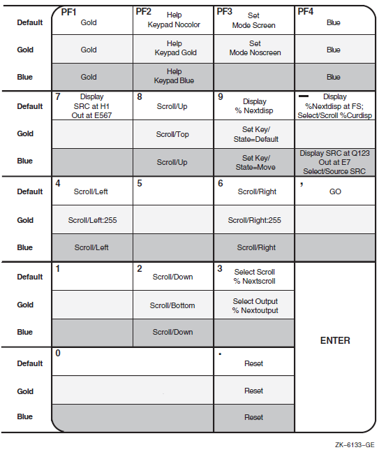
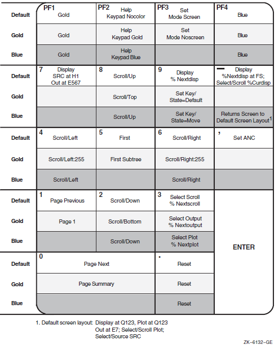
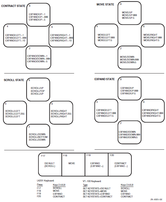
Appendix C. Questions and Answers
Why is 80% of my program in P1 space? How do I get the wait time reflected in code I can change?
When your program is waiting for a system service to complete, the program counter points to a location in the system service vector in P1 space. Because waiting for an I/O operation to complete is the most common form of system service wait, your program can appear to be spending most of its time in P1 space.
If your program does a lot of terminal I/O, you should expect the program to be I/O-bound and to appear to spend a lot of time in P1 space; the terminal is a slow device. If your program primarily does disk or tape I/O and appears to spend a lot of time in P1 space, investigate why the program is I/O-bound. By reprogramming your program's I/O to reduce the I/O wait time, you may be able to speed up your program considerably.
To get the system service wait time reflected in the code of your own program, gather stack PC values using the STACK_PC command in the Collector,then issue the PLOT or TABULATE command with the /MAIN_IMAGE qualifier to plot your data. This will charge the time outside your image (including that spent in P1 space) to the actual location within your image that caused the time to be spent.
How do I get the time spent in shareable images to be charged to the parts of my program that used it?
Gather stack PC data in the Collector and use the /MAIN_IMAGE qualifier with your PLOT command. This charges the time outside your image to the PC within the image that caused it.
How do I get the time spent in a specific RTL routine to be charged to the parts of my program that used it?
Gather stack PC data in the Collector, then issue the PLOT command with /MAIN_IMAGE=SHARE$RTL and /STACK =n qualifiers.
How can I find the specific instructions within a line that are taking the most time?
Use PLOT LINE module_name\%LINE nnn BY BYTE. Then, look at a machine listing to correlate byte offsets from the beginning of the line to the specific instructions.
How do I discard the time spent in terminal I/O?
Place an event marker before each terminal I/O statement and a different event marker after the terminal I/O statement. Then use SET FILTER foo TIME <> the_first_event_marker_name in the Analyzer. This discards all the time spent waiting for terminal I/O. See Chapter 4, "Productivity Enhancements with PCA" for an example of this.
When linked with PCA,why does my program ACCVIO before entering the Collector?
If the PCAC> prompt never appears, the Collector has probably not been installed as a privileged image. Possibly,the system manager forgot to edit the system startup file to include @SYS$STARTUP:PCA$STARTUP.COM. If the PCAC> prompt does appear, see question 7.
Why does my program behave differently when running with PCA?
One of the following conditions probably exists:Conditions 1 and 2 occur because PCA comes in as a handler and uses the stack above the user program's stack. Consequently, the stack is manipulated in ways that are different than when run without PCA. Although this is unlikely to happen, compiler code generation bugs have caused this sort of behavior.Uninitialized stack variables
Dependence on memory above SP
Assumptions about memory allocation
Condition 3 occurs because PCA now lives in the process memory space and requests memory by means of SYS$EXPREG. PCA requests a large amount of memory at initialization to minimize the altering of memory allocation, but this still may happen.
PCA may have a bug where it is smashing the stack or the random user memory. VSI appreciates your input on this because these bugs are hard to track down, and because they have been known to come and go based on the order of modules in a linker options file.
VSI recommends that you do the following:If you still believe that PCA is changing the behavior of your program, please submit an SPR with the following:Issue the GO/NOCOLLECT command. If the program does not behave as expected, the problem is your link with PCA.
Try a run with simple PC sampling only. PC sampling is the least likely mode for bugs. If your program does not behave as expected, the problem probably lies with your program. If your program behaves as expected, the problem probably lies with PCA.
A copy of the .EXE linked with PCA.
A command procedure which reproduces the problem using the above program.
Anything else you think VSI might find useful.
Why does it take so long to create a performance data file?
The Collector copies the portions of the DST it needs to the performance data file. This can take some time for large programs. The DST is placed in the performance datafile to avoid confusion over which image contains the DST for the data gathered. Also, PCA does not need all the information in the DST and condenses it. This avoids the overhead of reading useless information every time the file is used.
My application takes 10 days to compile. Is there a way I can avoid compiling my whole application with /DEBUG?
Yes. PCA provides all functionality except annotated source listings and codepath analysis, because all objects contain traceback information and most of the DST information that PCA needs is there. Once you find which modules are of interest, you can compile those with /DEBUG, then relink the application and gather the data again.
PCA tells me a large amount of time is being spent at a call instruction. Why? The call instruction should be a small part of the time spent executing the routine.
First, check page faulting. Sometimes the faulting behavior of a program causes a moderately called routine to get paged out just before it is called, and the page fault is a disk access. If that is not the case, check for JSB linkages to an RTL routine.
For performance reasons, some RTL routines use JSB linkages. This can cause confusion for the user when the /MAIN_IMAGE qualifier is used. This is especially true with PC sampling data, but can occur with any kind of data for which you can gather stack PC data.
Because a JSB linkage does not place a call frame on the stack, the return address to the site of the call is lost to PCA. Consequently, the first return address found by /MAIN_IMAGE is the site of the call to the routine that called the RTL by means of a JSB linkage. As an example, suppose routine MAIN called routine FOO, which in turn called the RTL by means of a JSB linkage. Then, suppose that a PC sampling hit occurred in the RTL. The PCs recorded are the actual PC when the hit occurred, the PC of the call to FOO, and the PC of the call to MAIN. Thus, in the presence of the /MAIN_IMAGE qualifier, the first PC within the image is the PC of the call to FOO. Consequently, FOO's call site is inflated by the number of data points in the RTL that are in routines that have JSB linkages.
This method can yield useful information. If you compare the time with /MAIN_IMAGE to the time without /MAIN_IMAGE, you can tell how much time was spent in JSB linkage routines. You cannot, however, separate the various JSB linkage routines. Note further that if the JSB routine is called from the main program, the data points will be lost because there is no caller of the main program.
Why does the Analyzer report 0.0% for a line and then output a full line of stars, indicating that the line was covered?
Probably, the total number of data points is over 2000,and the percentage is less than 0.05%. Therefore, rounding makes it 0.0%.
I have a utility routine that I have optimized as much as I can. I need to know who is calling it and how often, so I can reduce the number of calls to it. How do I get this information?
Use the PLOT command with the /MAIN_IMAGE = utility_routine qualifier to obtain the following options:PLOT CALL_TREE BY CHAIN_ROUTINE lists all the call chains that pass through utility_routine with the number of data points for each call chain. See Section 3.3.7, ''Using CALL_TREE Node Specifications''.
PLOT/STACK = 1 PROGRAM BY ROUTINE lists all the callers of utility_routine.
If one particular caller of utility_routine is of interest, try the following: SET FILTER filter_name CHAIN=(*,caller,utility_routine,*). This assures that the data being viewed is only that whose chains have a subchain caller, utility_routine.
Many other combinations of /CUMULATIVE, /MAIN_IMAGE, /STACK with various filters and nodespecs may be useful.
Why am I getting several coverage data points associated with my routine declaration when I do COVERAGE BY CODEPATH?
Several languages generate prologue code at each routine entry to initialize the language specific semantics. As far as PCA is concerned, code is code and deserves code path analysis. This environment is usually set up by a CALLS or JSB to an RTL routine. PCA considers CALLS, CALLG, and JSB to be transfers of control, because control does not in principle have to come back, and places a BPT in the instruction following.
Why are hexadecimal numbers showing up in the CALL_TREE plot?
The Analyzer was not able to symbolize the return address it found in the call stack. If I/O services or services data is being gathered, these may be addresses in the relocated system service vector.
How can I avoid all the source header information and get right to the most interesting line?
Use the traverse commands, NEXT, FIRST, PREVIOUS, CURRENT.
How can I easily compare different kinds of data?
Use the INCLUDE command, which uses a subset of PLOT qualifiers and parameters.
The Analyzer is running out of virtual memory. What do I do?
Raise the appropriate quotas, limit the number of displays, and limit the memory used by displays (use /SIZE=n).
Limit the size of your plots with the following methods:Use limiting nodespecs. For example, if PROGRAM_ADDRESS BY LINE does notwork, try MODULE foo BY LINE, or ROUTINE fee BY LINE.
Use the traverse commands after issuing PLOT/your_qualifiers PROGRAM_ADDRESS BY MODULE.
Use the /NOZEROS, /MINIMUM, /MAXIMUM qualifiers.
Use filters with CALL_TREE nodespecs to reduce the number of call chains.
Do not use the DECwindows interface.
The Collector is running out of virtual memory. What do I do?
If you are doing coverage or counter analysis, limit the number of breakpoint settings by using either MODULE BY LINE or CODEPATH node specifications instead of using PROGRAM BY LINE or do not use the DECwindows interface. Then do several collection runs to gather the data.
Why do some plots execute more quickly than others?
Some PLOT commands execute more quickly than others because PCA uses all available information from the previous plot to produce the requested one. For example, if you enter PLOT PROGRAM BY LINE and then enter PLOT/DESCENDING, PCA only sorts the previous plot. However, if you use a different nodespec, such as PLOT ROUTINE foo$bar BY CODEPATH, then PCA must rebuild its internal tables and read the data again, which takes more time. In addition, the number of filters and buckets you use affects the time it takes to build a plot. This is because filters affect the amount of data the Analyzer looks at, and because all buckets must be searched for each data point.
Why don't I see all my subroutine calls in a CALL_TREE plot?
It may be that you have a JSB linkage. See question 7.
Why do I get bad offsets when plotting MACRO modules by byte?
When plotting MACRO modules by byte, the offset is actually from the beginning of the module, including the data psects. You get bad offsets because the linker moves the psects around based on the psect attributes. Thus, the offsets you get may have no relationship to any listing you may have. However, if you use PLOT ROUTINE foo BY BYTE, then the offsets are from the beginning of the routine. (This only works if you have an .ENTRY foo … directive in your program.)
Can PCA measure shareable images activated "on the fly" with LIB$FIND_IMAGE_SYMBOL?
Yes, if you relink against the image you want to activate. PCA uses a structure built by the image activator to find all the shareable image information it needs. By relinking the image, the image activator knows about the image and LIB$FIND_IMAGE_SYMBOL will work.
Why do I get an undefined symbol error message when I use the hexadecimal number FF0?
PCA considers FF0 an identifier unless you precede it with a zero. Any hexadecimal number with the digits A through F must be preceded by a zero to be correctly interpreted by PCA.
Why do most of my PC samples land on instructions immediately after a time-consuming hardware instruction rather than the hardware instruction itself?
ASTs cannot be delivered during a hardware instruction. Therefore, when the AST fires to collect the PC sample, it is most likely to fire right after the time-consuming instruction. This behavior is apparent in MACRO.
These data-kind qualifiers work with TIME BY EVENT only.
These data-kind qualifiers work with TIME BY EVENT and with TIME BY [n] MSECS.
This is collected for disk I/O only, not terminal I/O.
Note that yes means the filter is applied to the given data kind. A blank means that it is not.
For /CPU_SAMPLING only