VSI OpenVMS Performance Management Manual
- Operating System and Version:
- VSI OpenVMS Alpha Version 8.4-2L1 or higher
VSI OpenVMS IA-64 Version 8.4-1H1 or higher
VSI OpenVMS x86-64 Version 9.2-2 or higher
Preface
This manual presents techniques for evaluating, analyzing, and optimizing performance on a system running OpenVMS. Discussions address such wide-ranging concerns as:
Understanding the relationship between work load and system capacity
Learning to use performance-analysis tools
Responding to complaints about performance degradation
Helping the site adopt programming practices that result in the best system performance
Using the system features that distribute the work load for better resource utilization
Knowing when to apply software corrections to system behavior—tuning the system to allocate resources more effectively
Evaluating the effectiveness of a tuning operation; knowing how to recognize success and when to stop
Evaluating the need for hardware upgrades
The manual includes detailed procedures to help you evaluate resource utilization on your system and to diagnose and overcome performance problems resulting from memory limitations, I/O limitations, CPU limitations, human error, or combinations of these. The procedures feature sequential tests that use OpenVMS tools to generate performance data; the accompanying text explains how to evaluate it.
Whenever an investigation uncovers a situation that could benefit from adjusting system values, those adjustments are described in detail, and hints are provided to clarify the interrelationships of certain groups of values. When such adjustments are not the appropriate or available action, other options are defined and discussed.
Decision-tree diagrams summarize the step-by-step descriptions in the text. These diagrams should also serve as useful reference tools for subsequent investigations of system performance.
This manual does not describe methods for capacity planning, nor does it attempt to provide details about using OpenVMS RMS features (hereafter referred to as RMS). Refer to the Guide to OpenVMS File Applications for that information. Likewise, the manual does not discuss DECnet for OpenVMS performance issues, because the VSI DECnet-Plus for OpenVMS Network Management Guide manual provides that information.
1. About VSI
VMS Software, Inc. (VSI) is an independent software company licensed by Hewlett Packard Enterprise to develop and support the OpenVMS operating system.
VSI seeks to continue the legendary development prowess and customer-first priorities that are so closely associated with the OpenVMS operating system and its original author, Digital Equipment Corporation.
2. Intended Audience
This manual addresses system managers and other experienced users responsible for maintaining a consistently high level of system performance, for diagnosing problems on a routine basis, and for taking appropriate remedial action.
3. Document Structure
This manual is divided into 13 chapters and 4 appendixes, each covering a related group of performance management topics as follows:
Chapter 1, "Performance Management" provides a review of workload management concepts and describes guidelines for evaluating user complaints about system performance.
Chapter 2, "Performance Options" lists post-installation operations for enhancing performance and discusses performance investigation and tuning strategies.
Chapter 3, "Memory Management Concepts" discusses OpenVMS memory management concepts.
Chapter 4, "Evaluating System Resources" explains how to use utilities and tools to collect and analyze data on your system’s hardware and software resources. Included are suggestions for reallocating certain resources should analysis indicate such a need.
Chapter 5, "Diagnosing Resource Limitations" outlines procedures for investigating performance problems.
Chapter 6, "Managing System Resources" describes how to evaluate system resource responsiveness.
Chapter 7, "Evaluating the Memory Resource" describes how to evaluate the performance of the memory resource and how to isolate specific memory resource limitations.
Chapter 8, "Evaluating the Disk I/O Resource" describes how to evaluate the performance of the disk I/O resource and how to isolate specific disk I/O resource limitations.
Chapter 9, "Evaluating the CPU Resource" describes how to evaluate the performance of the CPU resource and how to isolate specific CPU resource limitations.
Chapter 10, "Compensating for Resource Limitations" provides general recommendations for improving performance with available resources.
Chapter 11, "Compensating for Memory-Limited Behavior" provides specific recommendations for improving the performance of the memory resource.
Chapter 12, "Compensating for I/O-Limited Behavior" provides specific recommendations for improving the performance of the disk I/O resource.
Chapter 13, "Compensating for CPU-Limited Behavior" provides specific recommendations for improving the performance of the CPU resource.
Appendix A, "Decision Trees" lists the decision trees used in the various performance evaluations described in this manual.
Appendix B, "MONITOR Data Items" summarizes the MONITOR data items you will find useful in evaluating your system.
Appendix C, "MONITOR Multifile Summary Report" provides an example of a MONITOR multifile summary report.
Appendix D, "ODS–1 Performance Information" provides ODS-1 performance information.
4. Related Documents
For additional information on the topics covered in this manual, you can refer to the following documents:
VSI OpenVMS System Manager's Manual
Guide to OpenVMS File Applications
VSI OpenVMS System Management Utilities Reference Manual
Guidelines for OpenVMS Cluster Configurations
VSI OpenVMS Cluster Systems Manual
5. VSI Encourages Your Comments
You may send comments or suggestions regarding this manual or any VSI document by sending electronic mail to the following Internet address: <docinfo@vmssoftware.com>. Users who have VSI OpenVMS support contracts through VSI can contact <support@vmssoftware.com> for help with this product.
6. OpenVMS Documentation
The full VSI OpenVMS documentation set can be found on the VMS Software Documentation webpage at https://docs.vmssoftware.com.
7. Conventions
The following conventions are used in this manual:
| Convention | Meaning |
|---|---|
. . . | A vertical ellipsis indicates the omission of items from a code example or command format; the items are omitted because they are not important to the topic being discussed. |
| ( ) | In command format descriptions, parentheses indicate that you must enclose choices in parentheses if you specify more than one. |
| [ ] | In command format descriptions, brackets indicate optional choices. You can choose one or more items or no items. Do not type the brackets on the command line. However, you must include the brackets in the syntax for OpenVMS directory specifications and for a substring specification in an assignment statement. |
| | | In command format descriptions, vertical bars separate choices within brackets or braces. Within brackets, the choices are optional; within braces, at least one choice is required. Do not type the vertical bars on the command line. |
| bold type | This typeface represents the introduction of a new term. It also represents the name of an argument, an attribute, or a reason. |
| italic type | Italic text indicates important information, complete titles of manuals, or variables. Variables include information that varies in system output (Internal error number), in command lines (/PRODUCER=name), and in command parameters in text (where dd represents the predefined code for the device type). |
| UPPERCASE TYPE | Uppercase text indicates a command, the name of a routine, the name of a file, or the abbreviation for a system privilege. |
Monospace
text |
Monospace type indicates code examples and interactive screen displays. In the C programming language, monospace type in text identifies the following elements: keywords, the names of independently compiled external functions and files, syntax summaries, and references to variables or identifiers introduced in an example. |
| - | A hyphen at the end of a command format description, command line, or code line indicates that the command or statement continues on the following line. |
| numbers | All numbers in text are assumed to be decimal unless otherwise noted. Nondecimal radixes—binary, octal, or hexadecimal—are explicitly indicated. |
Chapter 1. Performance Management
Managing system performance involves being able to evaluate and coordinate system resources and workload demands.
CPU
Memory
Disk I/O
Network I/O
LAN I/O
Internet I/O
Cluster communication other than LAN (CI, FDDI, MC)
In addition to this manual, specific cluster information can be found in the Guidelines for OpenVMS Cluster Configurations and the VSI OpenVMS Cluster Systems Manual.
Acquiring a thorough knowledge of your work load and an understanding of how that work load exercises the system's resources
Monitoring system behavior on a routine basis in order to determine when and why a given resource is nearing capacity
Investigating reports of degraded performance from users
Planning for changes in the system work load or hardware configuration and being prepared to make any necessary adustments to system values
Performing certain optional system management operations after installation
A review of workload management concepts
Guidelines for developing a performance management strategy
Because many different networking options are available, network I/O is not formally covered in this manual. General performance concepts discussed here apply to networking, and networking should be considered within the scope of analyzing any system performance problem. You should consult the documentation available for the specific products that you have installed for specific guidelines concerning configuration, monitoring, and diagnosis of a networking product.
Similarly, database products are extremely complex and perform much of their own internal management. The settings of parameters external to OpenVMS may have a profound effect upon how efficiently OpenVMS is used. Thus, reviewing server application specific-material is a must if you are to efficiently understand and resolve a related performance issue.
1.1. System Performance Management Guidelines
Even if you are familiar with basic concepts discussed in this section, there are some details discussed that are specific to this process, so please read the entire section.
1.1.1. The Performance Management Process
Long term measurement and observation of your system is key to understanding how well it is working and is invaluable in identifying potential performance problems before they become so serious that the system grinds to a halt and it negatively affects your business. Thus, performance management should be a routine process of monitoring and measuring your systems to assure good operation through deliberate planning and resource management.
Systematically measuring the system
Gathering and analyzing the data
Evaluating trends
Archiving data to maintain a performance history
You will often observe trends and thus be able to address performance issues before they become serious and adversely affect your business operations. Should an unforeseen problem occur, your historical data will likely prove invaluable for pinpointing the cause and rapidly and efficiently resolving the problem. Without past data from your formerly well-running system, you may have no basis upon which to judge the value of the metrics you can collect on your currently poorly running system. Without historical data you are guessing; resolution will take much longer and cost far more.
Upgrades and Reconfigurations
Some systems are so heavily loaded that the cost of additional functionality of new software can push the system beyond the maximum load that the system was intended to handle and thus deliver unacceptable response times and throughput. If your system is running near its limit now during peak workload periods, you want to ensure that you take the steps necessary to avoid pushing your system beyond its limits when you cannot afford it.
Slow response times
Erratic system behavior
Unexplained system pauses, hangs, or crashes
If this is the case, you need a performance audit to determine your current workload and the resources necessary to adequately support your current and possibly future workloads. Implementing changes not specifically designed to increase such a system's capacity or reduce its workload can degrade performance further. Thus, investing in a performance audit will pay off by delivering you a more reliable, productive, available, and lower maintenance system.
Many factors involved in upgrades and reconfigurations contribute to increased resource consumption. Future workloads your system will be asked to support may be unforeseeable due to changes in the system, workload, and business.
Blind reconfiguration without measurement, analysis, modification, and contingency plans can result in serious problems. Significant increases in CPU, disk, memory, and LAN utilization demand serious consideration, measurement, and planning for additional workload and upgrades.
1.1.2. Conducting a Performance Audit
Evaluate whether your systems are viable candidates for proposed changes.
Identify modifications that must be made.
Insure that planned and implemented changes deliver expected results.
Characterize CPU, disk, memory, and LAN utilization on the systems under consideration before reconfiguration.
Measure system activity after an installation.
Measure, plan, understand, test, and confirm. To understand how system workloads vary, you should perform measurements for one week, if not longer, before installing your network
Take into account that workloads follow business cycles which vary predictably throughout the day, the week, the month, and the year. These variations may be affected by financial and legal deadlines as well as seasonal factors such as holidays and other cyclic activity.
Seek to identify periods of peak heavy loads (relatively long periods of heavy load lasting approximately five or more minutes). Understanding their frequency and the factors affecting them is key to successful system planning and management.
Peak Workloads and the Cyclic Nature of Workloads
You must first identify periods of activity during which you cannot afford to have system performance degrade and then measure overall system activity during these periods.
These periods will vary from system to system minute to minute, hour to hour, day to day, week to week, and month to month. Holidays and other such periods are often significant factors and should be considered. These periods depend upon the business cycles that the system is supporting.
If the periods you have identified as critical cannot be measured at this time, then measurements taken in the immediate future will have to be used as the basis for estimates of the activity during those periods. In such cases you will have to take measurements in the near term and make estimates based on the data you collect in combination with other data such as order rates from the previous calendar month or year, as well as projections or forecasts. But factors other than the CPU may become a bottleneck and slow down the system. For example, a fixed number of assistants can only process so many orders per hour, regardless of the number of callers waiting on the phone for service.
1.2. Strategies and Procedures
- Develop workload strategy (Chapter 1, "Performance Management")
Managing the work load
Distributing the work load
Sharing application code
- Develop tuning strategy (Chapter 2, "Performance Options")
Automatic Working Set Adjustment (AWSA)
AUTOGEN
Active memory management
- Perform general system resource evaluation (Chapter 4, "Evaluating System Resources")
CPU resource
Memory resource
Disk I/O resource
- Conduct a preliminary investigation of specific resource limitations (Chapter 5, "Diagnosing Resource Limitations")
Isolating memory resource limitations
Isolating disk I/O resource limitations
Isolating CPU resource limitations
- Review techniques for improving system resource responsiveness (Chapter 6, "Managing System Resources")
Providing equitable sharing of resources
Reducing resource consumption
Ensuring load balancing
Initiating offloading
- Apply specific remedy to compensate for resource limitations (Chapter 10, "Compensating for Resource Limitations")
Compensating for memory-limited behavior
Compensating for I/O-limited behavior
Compensating for CPU-limited behavior
1.3. System Manager's Role
Assume the responsibility for understanding the system's work load sufficiently to be able to recognize normal and abnormal behavior.
Predict the effects of changes in applications, operations, or usage.
Recognize typical throughput rates.
Evaluate system performance.
Perform tuning as needed.
1.3.1. Prerequisites
Be familiar with system tools and utilities.
Know your work load.
Develop a strategy for evaluating performance.
1.3.2. System Utilities and Tools
Accounting utility (ACCOUNTING)
Audit Analysis utility (ANALYZE/AUDIT)
Authorize utility (AUTHORIZE)
AUTOGEN command procedure
DCL SHOW commands
DECamds (Availability Manager)
DECevent utility (Alpha only)
Error Log utility (ANALYZE/ERROR_LOG)
Monitor utility (MONITOR)
On Alpha platforms, VSI recommends using the DECevent utility instead of the Error Log utility, ANALYZE/ERROR_LOG. (You invoke the DECevent utility with the DCL command, DIAGNOSE.) You can use ANALYZE/ERROR_LOG on Alpha systems, but the DECevent utility provides more comprehensive reports.
1.3.3. Why Use Them?
Collect and analyze key data items.
Observe usage trends.
Predict when your system reaches its capacity.
Adjust system parameters.
Modify users' privileges and quotas.
1.3.4. Knowing Your Work Load
What is the typical number of users on the system at each time of day?
What is the typical response time for various tasks for this number of users, at each hour of operation?
What are the peak hours of operation?
Which jobs typically run at which time of day?
Which commonly run jobs are intensive consumers of the CPU? of memory? of disk?
Which applications have the most image activations?
Which parts of the system software, if any, have been modified or user written, such as device drivers?
Are there any known system bottlenecks? Are there any anticipated ones?
Note
If you are a novice system manager, you should spend a considerable amount of time observing system operation using the DCL commands ACCOUNTING, MONITOR, and SHOW.
1.4. Developing a Strategy
Managing the work load
Distributing the work load
Sharing application code
1.4.1. Managing the Work Load
Is there a time of day when the work load peaks, that is, when it is noticeably heavier than at other times?
Is there any way to balance the work load better? Perhaps measures can be adopted by users.
Could any jobs be run better as batch jobs, preferably during nonpeak hours?
Have primary and secondary hours of operation been employed with users? Are the choices of hours the most appropriate for all users?
Can future applications be designed to work around any known or expected system bottlenecks? Can present applications be redesigned for the same purpose?
- Are you using all of the code-sharing features that the OpenVMS system offers you?
Note
Do not adjust any system values until you are satisfied that all these issues are resolved and that your workload management strategy is appropriate.
1.4.2. Distributing the Work Load
- Run large jobs as batch jobs.
Establish a site policy that encourages the submission of large jobs on a batch basis.
Regulate the number of batch streams so that batch usage is high when interactive usage is low.
Use DCL command qualifiers to run batch jobs at lower priority, adjust the working set sizes, and control the number of concurrent jobs.
For more information, see the VSI OpenVMS System Manager's Manual, Volume 1: Essentials.
- Restrict system use.
Do not permit more users to log in at one time than the system can support with adequate response time.
Restrict the number of interactive users with the DCL command SET LOGINS/INTERACTIVE.
Control the number of concurrent processes with the MAXPROCESSCNT system parameter.
Control the number of remote terminals allowed to access the system at one time with the RJOBLIM system parameter.
- Restrict system use to groups of users to certain days and hours of the day.
Use the Authorize utility to define permitted login hours for each user.
Use the DCL command SET DAY to override the conventional day-of-the-week associations for primary and secondary days.
- Design applications to reduce demand on binding resources.
Find out where system bottlenecks are located.
Plan use that minimizes demands on the bottleneck points.
1.4.3. Sharing Application Code
Application code sharing provides a cost-effective means of optimizing memory utilization. To ensure optimum performance of your system, make sure that frequently used code is shared.
Use the site-specific startup procedure to install as shared known images user-written programs and routines that are designed for sharing and have reached production status or are in general use.
Encourage programmers to write shareable code.
1.5. Analyzing Complaints
Ensure that hardware resources are adequate.
Know the work load reasonably well.
Have experience managing the work load according to the guidelines in Section 1.3.4, ''Knowing Your Work Load''.
1.5.1. Preliminary Steps
|
Step |
Action |
|---|---|
|
1 |
Obtain the following information:
|
|
2 |
Compare these facts with your knowledge of the normal work load and operation of your system. |
|
3 |
Follow the procedure shown in Figure A.1, ''Verifying the Validity of a Performance Complaint'' to verify the validity of the complaint. Did you observe the problem? Can you duplicate the problem? |
The following sections describe several reasons for performance problems.
1.5.2. Hardware Problem
|
Step |
Action |
|---|---|
|
1 |
Check the operator log and error log for indications of problems with specific devices. |
|
2 |
Enter the DCL commands SHOW ERROR and ANALYZE/ERROR_LOG to help determine if hardware is contributing to a performance problem. |
|
3 |
Review the previous day's error log as part of your morning routine. |
|
4 |
Obtain a count of errors logged since yesterday. Use the
following DCL command (which requires SYSPRV privilege):
For more information about error logging, see the VSI OpenVMS System Manager's Manual, Volume 2: Tuning, Monitoring, and Complex Systems; for information about using the Analyze/Error_Log utility, refer to the VSI OpenVMS System Management Utilities Reference Manual, Volume I: A–L. |
1.5.3. Blocked Process
A process enters the miscellaneous resource wait (MWAIT or RWAST) state usually because some resource, such as a paging file or mailbox, is unavailable (for example, because of a low quota or a program bug).
|
If... |
Then... |
|---|---|
|
A process is in the MWAIT state |
Use the DCL commands MONITOR PROCESSES and SHOW SYSTEM to identify the reason for the MWAIT state. |
|
The system fails to respond while you are investigating an MWAIT condition |
Check the system console for error messages. |
|
The MWAIT condition persists after you increase the capacity of the appropriate resource |
Investigate the possibility of a programming design error. |
1.5.4. Unrealistic Expectations
Users expect response times to remain constant, even as the system work load increases.
An unusual set of circumstances has caused exceptionally high demand on the system all at once.
Note
Whenever you anticipate a temporary workload change that will affect your users, notify them through broadcasts, text, or both, in the system notices.
Chapter 2. Performance Options
Poor operation
Lack of understanding of the work load and its operational ramifications
Lack of resources
Poor application design
Human error
A combination of these factors
Decompressing system libraries
Disabling file system high-water marking
Setting RMS file-extend parameters
Installing frequently used images
Enabling extended file caching
Reducing system disk I/O
Tuning
Note that not all the options discussed in this chapter are appropriate at every site.
2.1. Decompressing System Libraries
Most of the OpenVMS libraries are in compressed format in order to conserve disk space.
The CPU dynamically decompresses the libraries whenever they are accessed. However, the resulting performance slowdown is especially noticeable during link operations and when users are requesting online help.
If you have sufficient disk space, decompressing the libraries will improve CPU and elapsed-time performance.
Note
Decompressed object libraries take up about 25 percent more disk space than when compressed; the decompressed help libraries take up about 50 percent more disk space.
2.2. Disabling File System High-Water Marking
High-water marking is set by default whenever a volume is initialized. This security feature guarantees that users cannot read data they have not written.
How often new files are created
How often existing files are extended
How fragmented the volume is
- Enter a DCL command similar to the following:
$SET VOLUME/NOHIGHWATER_MARKING device-spec[:] Dismount and remount the volume.
2.3. Setting RMS File-Extend Parameters
Specifying larger values for system file-extend parameters
Setting the system parameter RMS_EXTEND_SIZE
Specifying a larger multiblock count
Specifying a larger multibuffer count
2.4. Installing Frequently Used Images
All processes use the same physical copy of the image.
The image will be activated in the most efficient way.
INSTALL ADD/OPEN/SHARED/HEADER_RESIDENT filename
INSTALL CREATE/OPEN/SHARED/HEADER_RESIDENT filename
ADD and CREATE are synonyms. The /SHARED and /HEADER_RESIDENT qualifiers imply the image is open. The /OPEN qualifier indicates the file is a permanently known image to the system.
2.5. Enabling File Caching
Enable extended file caching to reduce the number of disk I/O operations. See Section 12.2, ''Use Extended File Caching'' and the VSI OpenVMS System Manager's Manual.
2.6. Reducing System Disk I/O
|
Logical Name |
File |
|---|---|
|
ACCOUNTING |
System Accounting Data File |
|
AUDIT_SERVER |
Audit server master file |
|
QMAN$MASTER |
Job queue database master file ? |
|
Directory specification ? |
Job queue database queue and journal files |
|
NETPROXY |
NETPROXY.DAT |
|
OPC$LOGFILE_NAME |
Operator log files |
|
RIGHTSLIST |
RIGHTSLIST.DAT |
|
SYS$ERRORLOG |
ERRFMT log files |
|
SYS$JOURNAL |
DECdtm transaction log files |
|
SYS$MONITOR |
MONITOR log files |
|
SYSUAF |
SYSUAF.DAT |
|
VMSMAIL_PROFILE |
VMSMAIL_PROFILE.DATA |
In addition, the default DECNET account can reside on another disk. Refer to the DECNET record in the system authorization file.
You might consider moving paging and swapping activity off the system disk by creating large secondary page and swap files on a less heavily used disk.
In an educational or learning environment, there are several other files you might want to move off the system disk. If many users will frequently access the help libraries, you could move the directory pointed to by logical name SYS$HELP to another disk. However, the system installation and upgrade procedures assume SYS$HELP is on the system disk. If you move SYS$HELP to another disk, you will have to update it manually after a system upgrade.
If users frequently use computer-based instruction programs, you can move SYS$INSTRUCTION or DECW$CBI (or both) off the system disk, or make them into search lists.
Make these changes only if you have determined that the files in these directories are frequently used on your system.
2.7. Tuning
Tuning is the process of altering various system values to obtain the optimum overall performance possible from any given configuration and work load.
Note
When you have optimized your current system, the acquisition and installation of additional memory or devices can vastly improve system operation and performance.
Always aim for best overall performance, that is, performance viewed over time. The work load is constantly changing on most systems. Therefore, what guarantees optimal workload performance at one time might not produce optimal performance a short time later as the work load changes.
2.7.1. Prerequisites
Improper operation
Unreasonable performance expectations
Insufficient memory for the applications attempted
Inadequate hardware configuration for the work load, such as too slow a processor, too few buses for the devices, too few disks, and so forth
Improper device choices for the work load, such as using disks with insufficient speed or capacity
Hardware malfunctions
Poorly designed applications
Human error, such as allowing one process to consume all available resources
2.7.2. Tuning Suggestions
The effort required is often more expensive than a capacity upgrade.
The system includes AUTOGEN, which automatically establishes initial values for all system-dependent system parameters.
- The system includes features that in a limited way permit it to adjust itself dynamically during operation. The system can detect the need for adjustment in the following areas:
Nonpaged dynamic pool
Working set size
Number of pages on the free- and modified-page lists
As a result, these areas can grow dynamically, as appropriate, during normal operation. For more information on automatic adjustment features, see Section 3.5, ''Automatic Working Set Adjustment (AWSA)''. The most common cause of poor system performance is insufficient hardware capacity.
If you have adjusted your system for optimal performance with current resources and then acquire new capacity, you must plan to compensate for the new configuration. In this situation, the first and most important action is to execute the AUTOGEN command procedure.
If you anticipate a dramatic change in your workload, you should expect to compensate for the new workload.
2.7.3. Tools and Utilities
Caution
Do not directly modify system parameters using SYSGEN. AUTOGEN overrides system parameters set with SYSGEN, which can cause a setting to be lost months or years after it was made.
Use AUTHORIZE to change user account information, quotas, and privileges.
2.7.4. When to Use AUTOGEN
During a new installation or upgrade
Whenever your work load changes significantly
When you add an optional (layered) software product
When you install images with the /SHARED qualifier
On a regular basis to monitor changes in your system's work load
When you adjust system parameters
AUTOGEN will not fix a resource limitation.
2.7.5. Adjusting System Parameter Values
|
If you want to... |
Then... |
|---|---|
|
Modify system parameters |
Use the AUTOGEN command procedure. |
|
Change entries in the UAF |
Use AUTHORIZE. |
2.7.6. Using AUTOGEN Feedback
AUTOGEN has special features that allow it to make automatic adjustments for you in associated parameters. Periodically running AUTOGEN in feedback mode ensures that the system is optimally tuned.
The operating system keeps track of resource shortages in subsystems where resource expansion occurs. AUTOGEN in feedback mode uses this data to perform tuning.
2.7.7. Evaluating Tuning Success
|
Step |
Action |
|---|---|
|
1 |
Run a few programs that produce fixed and reproducible results at the same time you run your normal work load. |
|
2 |
Measure the running times. |
|
3 |
Adjust system values. |
|
4 |
Run the programs again at the same time you run your normal work load under nearly identical conditions as those in step 1. |
|
5 |
Measure the running times under nearly identical workload conditions. |
|
6 |
Compare the results. |
|
7 |
Continue to observe system behavior closely for a time after you make any changes. |
Note
This test alone does not provide conclusive proof of success. There is always the possibility that your adjustments have favored the performance of the image you are measuring—to the detriment of others.
2.7.7.1. When to Stop Tuning
In every effort to improve system performance, there comes a point of diminishing returns. After you obtain a certain level of improvement, you can spend a great deal of time tuning the system yet achieve only marginal results.
Because a system that has been improperly adjusted usually exhibits blatant symptoms with fairly obvious and simple solutions, you will likely find that tuning—in the form of adjustments to certain critical system values—produces a high return for the time and effort invested and that there is a much lower risk of error. As a guideline, if you make adjustments and see a marked improvement, make more adjustments and see about half as much improvement, and then fail to make more than a small improvement on your next attempt or two, you should stop and evaluate the situation. In most situations, this is the point at which to stop tuning.
2.7.7.2. Still Not Satisfied?
If you are not satisfied with the final performance, consider increasing your capacity through the addition of hardware.
Generally, memory is the single piece of hardware needed to solve the problem. However, some situations warrant obtaining additional disks or more CPU power.
Chapter 3. Memory Management Concepts
The operating system employs several memory management mechanisms and a memory reclamation policy to improve performance on the system. These features are enabled by default. In the majority of situations, they produce highly desirable results in optimizing system performance. However, under rare circumstances, they might contribute to performance degradation by incurring their own overhead. This chapter describes these features and provides insight into how to adjust, or even turn them off, through tuning.
3.1. Memory
Once you have taken the necessary steps to manage your work load, you can evaluate reports of performance problems. Before you proceed, however, it is imperative that you be well versed in the concepts of memory management.
On OpenVMS VAX, system parameter values are allocated in units of 512-byte pages. On OpenVMS Alpha, some system parameter values are allocated in units of pages, while others are allocated in units of pagelets. (A pagelet is equal to a VAX page, or 512 bytes.) Figure 3.1, ''OpenVMS Memory Configuration'' illustrates the configuration of memory for OpenVMS systems.
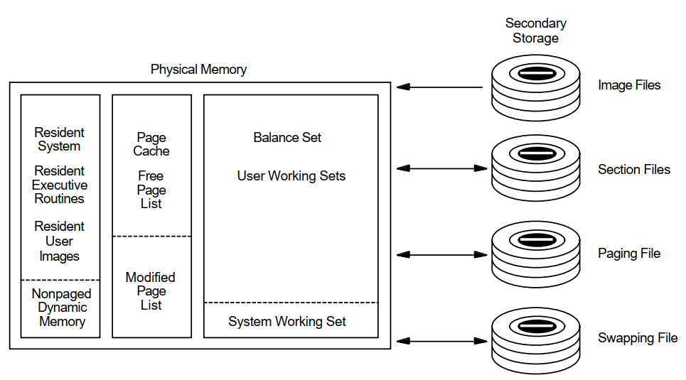 |
3.1.1. Physical Memory
Primary page cache where processes execute: the balance set resides in the primary page cache.
- Secondary page cache where data is stored for movement to and from the disks. The secondary page cache consists of two sections as follows:
Free-page list—Pages whose contents have not been modified
Modified-page list—Pages whose contents have been modified
Operating system resident executive.
Each disk has only one access path available to transfer data from and to physical memory, that is, to perform disk I/O.
3.1.2. Virtual Memory
Physical memory
Secondary storage (disk)
From the programmer's point of view, the secondary storage locations appear to be locations in physical memory.
3.1.3. Process Execution Characteristics
A process executes in physical memory until it must wait—usually for the completion of an I/O request.
Every time a process has to wait, another process may use the CPU.
The operating system maintains an even balance in the use of memory, CPU time, and the number of processes running at once.
- Each time a process starts to execute, it is assigned a slice of computer processing time called a quantum. The process will continue to execute until one of three possible events occurs:
A higher priority process becomes executable. In this case the lower priority process is preempted and the higher priority process starts to execute.
The process enters a wait state, for example, in order to wait for the completion of an I/O operation.
The assigned quantum expires. If no other process of equal or higher priority is ready to execute, the current process obtains a new quantum and continues execution. If another process of equal priority is already waiting to execute, the current process must now wait and the new process obtains the CPU for the duration of 1 quantum.
This round-robin mode of scheduling does not apply to real-time processes. They cannot be interrupted by other processes of equal priority.
3.2. Working Set Paging
When... | Then... |
|---|---|
Image activation begins | The process brings in the first set of pages from the image file and uses them in its own working set. |
The process's demand for pages exceeds those available in the working set | Some of the process's pages must be moved to the page cache to make room or the process's working set is expanded. |
The page cache fills up | The swapper transfers a cluster of pages from the modified-page cache to a paging file. |
A hard fault requires a read operation from a page or image file on disk.
A soft fault involves mapping to a secondary page cache; this can be a global page or a page in the secondary page cache.
3.3. Process Swapping
When a process whose working set is in memory becomes inactive, the entire working set or part of it may be removed from memory to provide space for another process's working set to be brought in for execution.
Swapping is the partial or total removal of a process's working set from memory.
3.3.1. What Is the Swapper?
The swapper process schedules physical memory. It keeps track of the pages in both physical memory and on the disk paging and swapping files so it can ensure that each process has a steady supply of pages for each job.
3.3.2. Types of Swapping
Swapper trimming—Pages are removed from the target working set but the working set is not swapped out.
Process swapping—All pages are swapped out of memory.
3.4. Initial Working Set Quotas and Limits
The memory management strategy depends initially on the values in effect for the working set quota (WSQUOTA) and working set extent limit (WSEXTENT).
3.4.1. Processes
When a process is created, its quota and related limits must be specified. The LOGINOUT facility obtains the parameter settings for the quota and related limits from the record in the user authorization file (UAF) that characterizes the user. (System managers create a UAF record for each user.) LOGINOUT is run when a user logs in and when a batch process starts.
When an interactive job runs, the values in effect might have been lowered or raised either by the corresponding qualifiers on the last SET WORKING_SET command to affect them, or by the system service $ADJWSL.
The initial size of a process's working set is defined (in pagelets) by the process's working set default quota WSDEFAULT.
When ample memory is available, a process's working set upper growth limit can be expanded to its working set extent, WSEXTENT.
3.4.2. Subprocesses and Detached Processes
$CREPRC system service
DCL command RUN
|
Parameter |
Characteristic |
|---|---|
|
PQL_DWSDEFAULT |
Default WSDEFAULT |
|
PQL_DWSQUOTA |
Default WSQUOTA |
|
PQL_DWSEXTENT |
Default WSEXTENT |
|
PQL_MWSDEFAULT |
Minimum WSDEFAULT |
|
PQL_MWSQUOTA |
Minimum WSQUOTA |
|
PQL_MWSEXTENT |
Minimum WSEXTENT |
AUTOGEN checks all these values and overrides them if the values in the UAF are too large or too small.
PQL parameters are described in the VSI OpenVMS System Management Utilities Reference Manual.
3.4.3. Batch Queues
When a batch queue is created, the DCL command INITIALIZE/QUEUE establishes the default values for jobs with the /WSDEFAULT, /WSQUOTA, and /WSEXTENT qualifiers.
However, you can set these qualifiers to defer to the user's values in the UAF record.
When a batch job runs, the values may have been lowered by the corresponding qualifiers on the DCL commands SUBMIT or SET QUEUE/ENTRY.
3.4.4. Required Memory Resources
Small (Up to 200 pages) — For editing, and for compiling and linking small programs (typical interactive processing)
Large (400 or more pages) — For compiling and linking large programs, and for executing programs that manipulate large amounts of data in memory (typical batch processing)
Note that the definitions of "small" and "large" working sets change with time, and the memory required may increase with the addition of new features to programs. Furthermore, many applications now take advantage of the increased memory capacity of newer Alpha systems and the increased addressing space available to programs. Applications, especially database and other data handling programs, may need much larger working sets than similar applications required in the past.
Small (256 to 800 pages) — For editing, and for compiling and linking small programs (typical interactive processing)
Large (1024 pages or more) — For compiling and linking large programs, and for executing programs that manipulate large amounts of data in memory (typical batch processing)
3.4.5. User Programs
Working set limits for user programs depend on the code-to-data ratio of the program and on the amount of data in the program.
Programs that manipulate mostly code and that either include only small or moderate amounts of data or use RMS to process data on a per-record basis require only a small working set.
Programs that manipulate mostly data such as sort procedures, compilers, linkers, assemblers, and librarians require a large working set.
3.4.6. Guidelines
System parameters—Set WSMAX at the highest number of pages required by any program.
- UAF options
Set WSDEFAULT at the median number of pages required by a program that the user will run interactively.
Set WSQUOTA at the largest number of pages required by a program that the user will run interactively.
Set WSEXTENT at the largest number of pages you anticipate the process will need. Be as realistic as possible in your estimate.
- Batch queues for user-submitted jobs
Set WSDEFAULT at the median number of pages required.
Set WSQUOTA to the number of pages that will allow the jobs to complete within a reasonable amount of time.
Set WSEXTENT (using the DCL command INITIALIZE/QUEUE or START/QUEUE) to the largest number of pages required.
This arrangement effectively forces users to submit large jobs for batch processing because otherwise, the jobs will not run efficiently. To further restrict the user who attempts to run a large job interactively, you can impose CPU time limits in the UAF.
3.5. Automatic Working Set Adjustment (AWSA)
The automatic working set adjustment (AWSA) feature allows processes to acquire additional working set space (physical memory) under control of the operating system.
This activity reduces the amount of page faulting.
By reviewing the need for each process to add some pages to its working set limit (based on the amount of page faulting), the operating system can better balance the working set space allocation among processes.
3.5.1. What Are AWSA Parameters?
The AWSA mechanism depends heavily on the values of the key system parameters: PFRATH, PFRATL, WSINC, WSDEC, QUANTUM, AWSTIME, AWSMIN, GROWLIM, and BORROWLIM.
Note
The possibility that AWSA parameters are out of balance is so slight that you should not attempt to modify any of the key parameter values without a very thorough understanding of the entire mechanism.
3.5.2. Working Set Regions
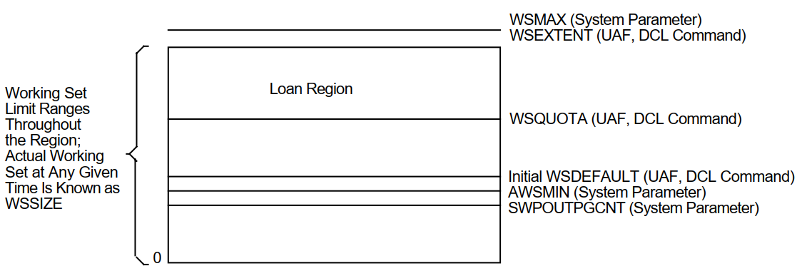
All processes have an initial default limit of pages of physical memory defined by the system parameter WSDEFAULT.
Any process that needs more memory is allowed to expand to the amount of a larger limit known as the working set quota defined by WSQUOTA.
Because page faulting is costly, the operating system has another feature for extending working set space to needy processes, provided the system has free memory available. If the conditions are right, the process can borrow working set space up to a final limit known as its working set extent, or WSEXTENT.
Whenever a process's working set size increases, the growth occurs in increments according to the value of the system parameter, WSINC.
Figure 3.2, ''Working Set Regions for a Process'' illustrates these important regions.
 |
3.5.3. Adjustment Period
The system recognizes or reviews the need for growth by sampling the page faulting rate of each process over an adjustment period. The adjustment period is the time from the start of the quantum (defined by the system parameter QUANTUM) right after an adjustment occurs until the next quantum after a time interval specified by the parameter AWSTIME elapses. For example, if the system quantum is 200 milliseconds and AWSTIME is 700 milliseconds, the system reviews the need to add or subtract pages from a process every time the process consumes 800 milliseconds of CPU time, or every fourth quantum.
3.5.4. How Does AWSA Work?
|
Stage |
Description | |
|---|---|---|
|
1 |
The system samples the page faulting rate of each process during the adjustment period. | |
|
2 |
The system parameters PFRATL and PFRATH define the upper and lower limits of acceptable page faulting for all processes. At the end of each process's adjustment period, the system reviews the need for growth and does the following: | |
|
Too high compared with PFRATH |
Approves an increase in the working set size of that process in the amount of system parameter WSINC up to the value of its WSQUOTA. | |
|
Too low compared with PFRATL (when PFRATL is nonzero) |
Approves a decrease in the working set size of that process in the amount of system parameter WSDEC. No process will be reduced below the size defined by AWSMIN. This process is called voluntary decrementing. | |
|
3 |
If the increase in working set size puts the process above the value of WSQUOTA and thus requires a loan, the system compares the availability of free memory with the value of BORROWLIM. The AWSA feature allows a process to grow above its WSQUOTA value only if there are at least as many pages of free memory as specified by BORROWLIM. If too many processes attempt to add pages at once, an additional mechanism is needed to stop the growth while it is occurring. However, the system only stops the growth of processes that have already had the benefit of growing beyond their quota. | |
|
If... |
Then the system... | |
|
A process page faults after its working set count exceeds WSQUOTA |
Examines the value of the parameter GROWLIM before it allows the process to use more of its WSINC loan. Note that this activity is not tied into an adjustment period but is an event-driven occurrence based on page faulting. | |
|
The number of pages on the free-page list is at least equal to or greater than GROWLIM |
Continues to allow the process to add pages to its working set. | |
|
The number of free pages is less than GROWLIM |
Will not allow the process to grow; the process must give back some of its pages before it reads in new pages. | |
|
Active memory reclamation is enabled |
Sets BORROWLIM and GROWLIM to very small values to allow active processes maximum growth potential. | |
3.5.5. Page Fault Rates
Page fault rate varies as a function of the working set size for a program. For initial working set sizes that are small relative to the demands of the program, a small increase in working set size results in a very large decrease in page fault rate. Conversely, as initial working set size increases, the relative benefit of increased working set size diminishes. Figure 3.3, ''Effect of Working Set Size on Page Fault Rate'' shows that by increasing the working set size in the example from 50 to 100 pages, the page fault rate drops from 200 to 100 pf/s. In the midrange the program still benefits from an increase in its working set, but in this realm twice the increase in the working set (100 to 200 pages versus 50 to 100 pages) yields only half the decrease in page fault rate (100 to 50 pf/s versus 200 to 100 pf/s). A point may be reached at which further substantial increases in working set size yields little or no appreciable benefit.
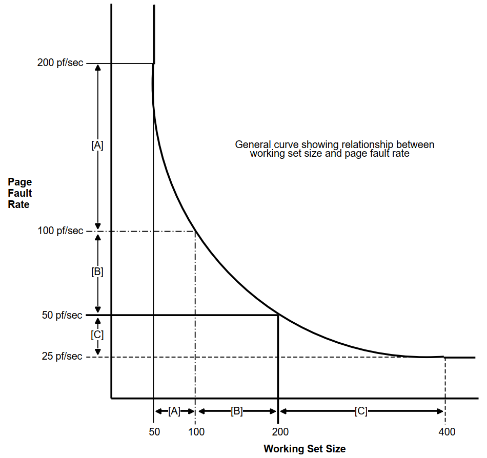 |
Figure 3.3, ''Effect of Working Set Size on Page Fault Rate'' illustrates a general relationship between working set size and page fault rate. The numbers provided are for comparison only. Not all programs exhibit the same curve depicted. Three different ranges are delineated to show that the effect of increasing working set size can vary greatly depending upon a program's requirements and initial working set size.
Figure 3.4, ''Setting Minimum and Maximum Page Fault Rates'' illustrates setting minimum and maximum page fault rates and determining the required working set size for images running on your system.
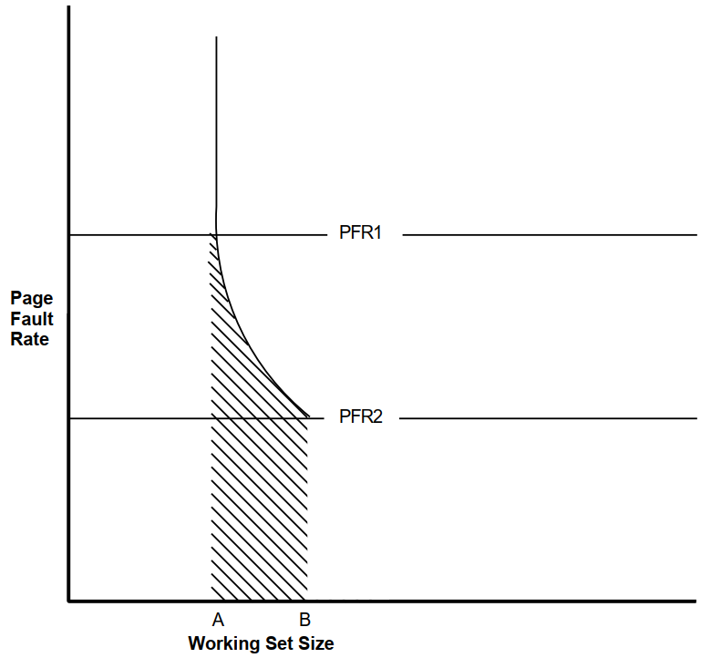 |
If... | Then... |
|---|---|
You establish a maximum acceptable page fault rate of PFR1 | For each image there is a minimum required working set size as shown at point A in Figures 3.3 and 3.4. |
You determine that the minimum level of page faulting is defined by PFR2 for all images | For each image there is a point (shown at point B) that is the maximum size the working set needs to reach. |
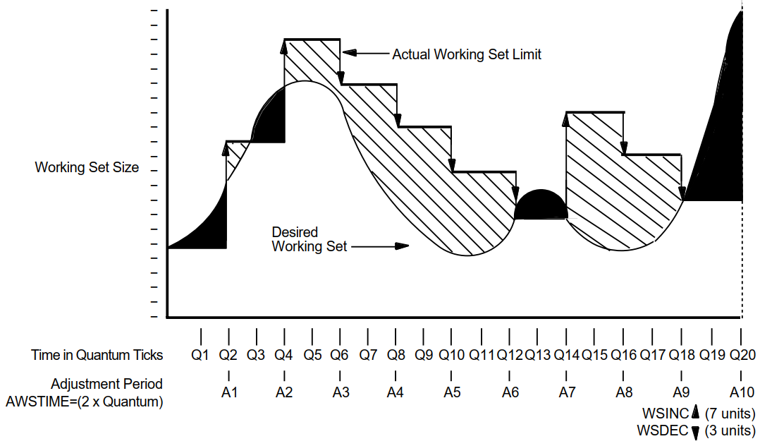
Figure 3.5, ''An Example of Working Set Adjustment at Work'' illustrates how automatic working set adjustment works over time, across the whole system, to minimize the amount of page faulting by adjusting working set sizes in balance with the amount of free memory available. The units used for AWSTIME, WSDEC, and WSINC in Figure 3.5, ''An Example of Working Set Adjustment at Work'' are for illustration; they are not recommendations.
In the figure, the shaded area identifies where paging occurs. The portion between the desired working set size and the actual working set limit (shown with cross-hatching) represents unnecessary memory overhead—an obvious instance where it costs memory to minimize page faulting.
 |
3.5.6. Voluntary Decrementing
The parameters PFRATL and WSDEC, which control voluntary decrementing, are very sensitive to the application work load.
For the PFRATH and PFRATL parameters, it is possible to define values that appear to be reasonable page faulting limits but yield poor performance.
The problem results from the page replacement algorithm and the time spent maintaining the operation within the page faulting limits.
For example, for some values of PFRATL, you might observe that a process continuously page faults as its working set size grows and shrinks while the process attempts to keep its page fault rate within the limits imposed by PFRATH and PFRATL.
However, you might observe the same process running in approximately the same size working set, without page faulting once, with PFRATL turned off (set to zero).
Oscillation occurs when a process's working set size never stabilizes. To prevent the site from encountering an undesirable extreme of oscillation, the system turns off voluntary decrementing by initially setting parameter PFRATL equal to zero. You will achieve voluntary decrementing only if you deliberately turn it on.
3.5.7. Adjusting AWSA Parameters
|
Task |
Adjustment |
|---|---|
|
Enable voluntary decrementing |
Set PFRATL greater than zero. |
|
Disable borrowing |
Set WSQUOTA equal to WSEXTENT. |
|
Disable AWSA (per process) |
Enter the DCL command SET WORKING_SET/NOADJUST. |
|
Disable AWSA (systemwide) |
Set WSINC to zero. |
Note
If you plan to change any of these AWSA parameters, review the documentation for all of them before proceeding. You should also be able to explain why you want to change the parameters or the system behavior that will occur. In other words, never make whimsical changes to the AWSA parameters on a production system.
3.5.8. Caution
You can circumvent the AWSA feature by using the DCL command SET WORKING_SET/NOADJUST.
Use caution in disabling the AWSA feature, because conditions could arise that would force the swapper to trim the process back to the value of the SWPOUTPGCNT system parameter.
Once AWSA is disabled for a process, the process cannot increase its working set size after the swapper trims the process to the SWPOUTPGCNT value. If the value of SWPOUTPGNT is too low, the process is restricted to that working set size and will fault badly.
3.5.9. Performance Management Strategies for Tuning AWSA
By developing a strategy for performance management that considers the desired automatic working set adjustment, you will know when the AWSA parameters are out of adjustment and how to direct your tuning efforts.
- Rapid response—Tune to provide a rapid response whenever the load demands greater working set sizes, allowing active memory reclamation to return memory from idle processes. To implement this strategy:
Start processes off with small values for their working set defaults.
Set PFRATH low (possibly even to zero).
Set a low value for AWSTIME.
Set a relatively large value for WSINC.
Set BORROWLIM low and WSEXTENT high (even as high as WSMAX) to provide either large working set quotas or generous loans.
This is the default OpenVMS strategy where both BORROWLIM and GROWLIM are set equal to the value of FREELIM to allow maximum growth by active processes, and active reclamation is enabled to return memory idle processes.
- Less dynamic response—Tune for a less dynamic response that will stabilize and track moderate needs for working set growth. To implement this strategy:
Establish moderate values for AWSTIME, WSINC, and PFRATH. For example, set WSINC equal to approximately 10 percent of the typical value for WSDEFAULT.
Provide more generous working set defaults, so that you do not need to set BORROWLIM so low as to ensure that loans would always be granted.
The first strategy works best in the time-sharing environment where there can be wild fluctuations in demand for memory from moment to moment and where there tends to be some number of idle processes consuming memory at any moment. The second strategy works better in a production environment where the demand tends to be more predictable and far less volatile.
3.6. Swapper Trimming
The swapper process performs two types of memory management activities—swapping and swapper trimming. Swapping is writing a process to a reserved disk file known as a swapping file, so that the remaining processes can benefit from the use of memory without excessive page faulting.
To better balance the availability of memory resources among processes, the operating system normally reclaims memory through a more complicated sequence of actions known as swapper trimming.
|
Stage |
Description | |
|---|---|---|
|
1 |
The system detects too few pages (below the value of FREELIM) in the free-page list. | |
|
2 |
The system checks whether a minimum number of pages exists in the modified-page list as defined by system parameter MPW_THRESH. | |
|
If... |
Then the system... | |
|
The minimum exists in the modified-page list |
Invokes the modified-page writer to write out the modified-page list and free its pages for the free-page list. | |
|
The modified-page list does not contain enough pages to match FREEGOAL |
Does not invoke the modified-page writer, but concludes that some of the processes should be trimmed; that is, forced to relinquish some of their pages or else be swapped out. | |
Trimming takes place at two levels (at process level and systemwide) and occurs before the system resorts to swapping.
3.6.1. First-Level Trimming
The swapper performs first-level trimming by checking for processes with outstanding loans; that is, processes that have borrowed on their working set extent. Such processes can be trimmed, at the swapper's discretion, back to their working set quota.
3.6.2. Second-Level Trimming
If first-level trimming failed to produce a sufficient number of free pages, then the swapper can trim at the second level.
With second-level trimming, the swapper refers to the systemwide trimming value SWPOUTPGCNT. The swapper selects a candidate process and then trims the process back to SWPOUTPGCNT and outswaps it. If the deficit is still not satisfied, the swapper selects another candidate.
As soon as the needed pages are acquired, the swapper stops trimming on the second level.
3.6.3. Choosing Candidates for Second-Level Trimming
Because the swapper does not want to trim pages needed by an active process, it selects the processes that are candidates for second-level trimming based on their states.
Memory is always reclaimed from suspended processes before it is taken from any other processes. The actual algorithm used for the selection in each of these cases is complex, but those processes that are in either local event flag wait or hibernate wait state are the most likely candidates.
|
Stage |
Description |
|---|---|
|
1 |
The swapper compares the length of real time that a process has been waiting since entering the hibernate (HIB) or local event flag wait (LEF) state with the system parameter LONGWAIT. |
|
2 |
From its candidate list, the system selects the better processes for outswapping that have been idle for a time period equal to or greater than LONGWAIT. |
By freeing up pages through outswapping, the system should allow enough processes to satisfy their CPU requirements, so that those processes that were waiting can resume execution sooner.
Dormant process pseudoclass
The process must be a nonreal-time process whose current priority is equal to or less than the system parameter DEFPRI (default 4).
The process must be a computable process that has not had a significant event (page fault, direct or buffered I/O, CPU time allocation) within an elapsed time period defined by the system parameter DORMANTWAIT (default 10 seconds).
3.6.4. Disabling Second-Level Trimming
To disable second-level trimming, increase SWPOUTPGCNT to such a large value that second-level trimming is never permitted.
The swapper will still trim processes that are above their working set quotas back to SWPOUTPGCNT, as appropriate.
If you encounter a situation where any swapper trimming causes excessive paging, it may be preferable to eliminate second-level trimming and initiate swapping sooner. In this case, tune the swapping with the SWPOUTPGCNT parameter.
For a process with the PSWAPM privilege, you can also disable swapping and second-level trimming with the DCL command SET PROCESS/NOSWAPPING.
3.6.5. Swapper Trimming Versus Voluntary Decrementing
Swapper trimming occurs on an as-needed basis.
Voluntary decrementing occurs on a continuous basis and affects only active, computable processes.
Voluntary decrementing can reach a detrimental condition of oscillation.
The AUTOGEN command procedure, which establishes parameter values when the system is first installed, provides for swapper trimming but disables voluntary decrementing.
3.7. Active Memory Reclamation from Idle Processes
The memory management subsystem includes a policy that actively reclaims memory from inactive processes when a deficit is first detected but before the memory resource is depleted.
Long-waiting processes
Periodically waking processes
3.7.1. Reclaiming Memory from Long-Waiting Processes
A candidate process for this policy would be in the LEF or HIB state for longer than number of seconds specified by the system parameter LONGWAIT.
First-Level Trimming
By setting FREEGOAL to a high value, memory reclamation from idle processes is triggered before a memory deficit becomes crucial and thus results in a larger pool of free pages available to active processes. When a process that has been swapped out in this way must be swapped in, it can frequently satisfy its need for pages from the large free-page list.
The system uses standard first-level trimming to reduce the working set size.
Second-Level Trimming
Second-level trimming with active memory reclamation enabled occurs, but with a significant difference.
When shrinking the working set to the value of SWPOUTPGCNT, the active memory reclamation policy removes pages from the working set but leaves the working set size (the limit to which pages can be added to the working set) at its current value, rather than reducing it to the value of SWPOUTPGCNT.
In this way, when the process is outswapped and eventually swapped in, it can readily fault the pages it needs without rejustifying its size through successive adjustments to the working set by AWSA.
Swapping Long-Waiting Processes
Long-waiting processes are swapped out when the size of the free-page list drops below the value of FREEGOAL.
A candidate long-waiting process is selected and outswapped no more than once every 5 seconds.
3.7.2. Reclaiming Memory from Periodically Waking Processes
Wake periodically
Do minimal work
Return to a sleep state
Watchdog Processes
Because it has a periodically waking behavior, a watchdog process is not a candidate for swapping but might be a good candidate for memory reclamation (trimming).
For this type of process, the policy tracks the relative wait-to-execution time.
How Trimming Is Performed
When the active memory reclamation policy is enabled, standard first- and second-level trimming are not used.
When the size of the free-page list drops below twice the value of FREEGOAL, the system initiates memory reclamation (trimming) of processes that wake periodically.
If a periodically waking process is idle 99 percent of the time and has accumulated 30 seconds of idle time, the policy trims 25 percent of the pages in the process's working set as the process reenters a wait state. Therefore, the working set remains unchanged.
3.7.3. Setting the FREEGOAL Parameter
The system parameter FREEGOAL controls how much memory is reclaimed from idle processes.
Setting FREEGOAL to a larger value reclaims more memory; setting FREEGOAL to a smaller value reclaims less.
For information about AUTOGEN and setting system parameters, refer to the VSI OpenVMS System Manager's Manual, Volume 2: Tuning, Monitoring, and Complex Systems.
3.7.4. Sizing Paging and Swapping Files
Because it reclaims memory from idle processes by trimming and swapping, the active memory reclamation policy can increase paging and swapping file use.
Use AUTOGEN in feedback mode to ensure that your paging and swapping files are appropriately sized for the potential increase.
For information about sizing paging and swapping files using AUTOGEN, refer to the VSI OpenVMS System Manager's Manual, Volume 2: Tuning, Monitoring, and Complex Systems.
3.7.5. How Is the Policy Enabled?
Active memory reclamation is enabled by default.
By using the system parameter MMG_CTLFLAGS which is bit encoded, you can enable and disable proactive memory reclamation mechanisms.
|
Bit ? |
Meaning |
|---|---|
|
<0> |
If this bit is set, reclamation is enabled by trimming from periodically executing but otherwise idle processes. This occurs when the size of the free list drops below two times FREEGOAL. Otherwise, if clear, it disables it. |
|
<1> |
If this bit is set, reclamation is enabled by outswapping processes that have been idle for longer than LONGWAIT seconds. This occurs when the size of the free list drops below FREELIM. Otherwise, if clear, it disables it. |
|
<2-7> |
Reserved for future use. |
MMG_CTLFLAGS is a dynamic parameter and is affected by AUTOGEN.
3.8. Memory Sharing
Memory sharing allows multiple processes to map to (and thereby gain access to) the same pages of physical memory.
Memory sharing (either code or data) is accomplished using a systemwide global page table similar in function to the system page table.
3.8.1. Global Pages
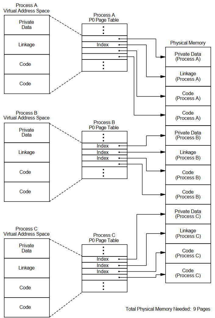
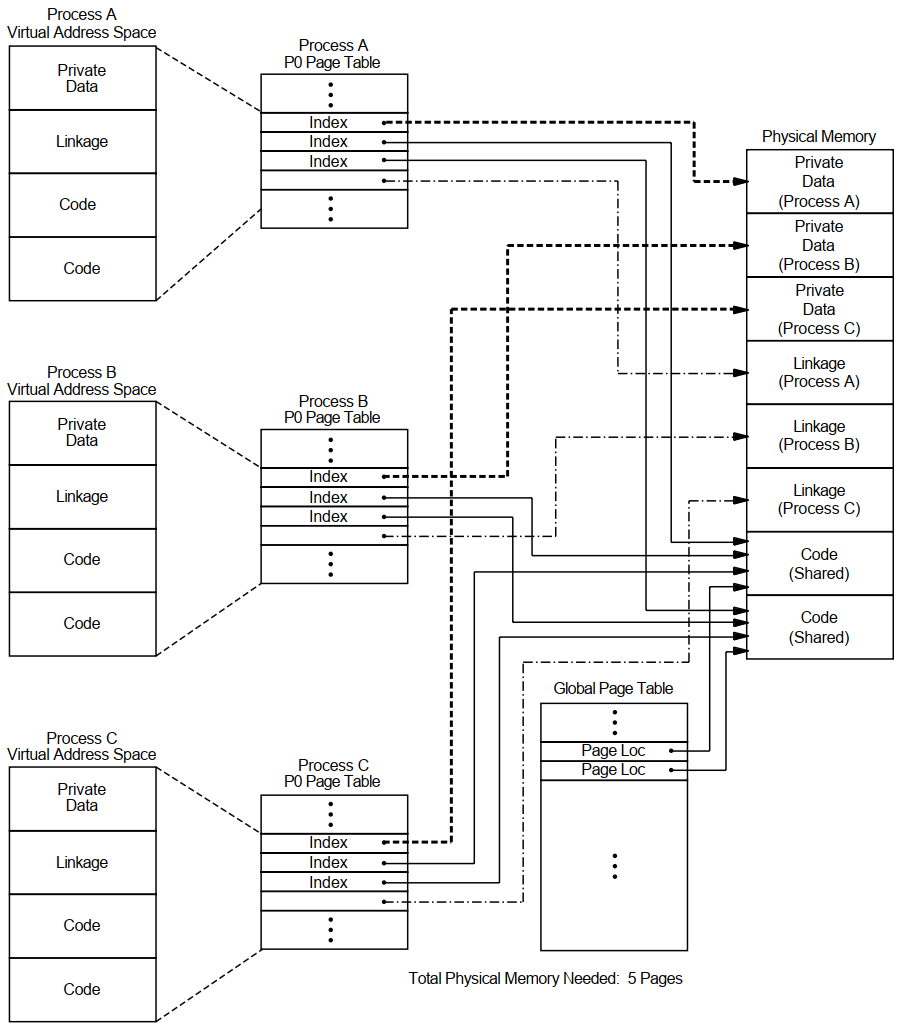
Figures 3.6 and 3.7 illustrate how memory can be conserved through the use of global (shared) pages. The three processes (A, B, and C) run the same program, which consists of two pages of read-only code and one page of writable data.
Figure 3.6, ''Example Without Shared Code'' shows the virtual-to-physical memory mapping required when each process runs a completely private copy of the program. Figure 3.7, ''Example with Shared Code'' illustrates the physical-memory gains possible and the data-structure linkage required when the read-only portion of the program is shared by the three processes. Note that each process must still maintain a private data area to avoid corrupting the data used by the other processes.
 |
 |
The amount of memory saved by sharing code among several processes is shown in the following formula:

For example, if 30 users share 300 pages of code, the savings are 8700 pages.
3.8.2. System Overhead
Each... | Requires a... | Allocated from the... |
|---|---|---|
Global page | Global page table entry | Global page table |
Global section | Global section table entry Global section descriptor | Global section table Paged dynamic pool |
For more information about global sections, see the VSI OpenVMS Linker Utility Manual.
3.8.3. Controlling the Overhead
GBLPAGES—Defines the size of the global page table. The system working set size as defined by SYSMWCNT must be increased whenever you increase GBLPAGES.
GBLSECTIONS—Defines the size of the global section table.
3.8.4. Installing Shared Images
Once an image has been created, it can be installed as a permanently shared image. (See the VSI OpenVMS Linker Utility Manual and the VSI OpenVMS System Manager's Manual, Volume 2: Tuning, Monitoring, and Complex Systems). This will save memory whenever there is more than one process actually mapped to the image at a time.
Also, use AUTHORIZE to increase the user's working set characteristics (WSDEF, WSQUO, WSEXTENT) wherever appropriate, to correspond to the expected use of shared code. (Note, however, that this increase does not mean that the actual memory usage will increase. Sharing of code by many users actually decreases the memory requirement.)
3.8.5. Verifying Memory Sharing
- Invoke the OpenVMS Install utility (INSTALL) and enter the LIST/FULL command. For example:
$INSTALLINSTALL>LIST/FULL LOGINOUTINSTALL displays information in the following format:DISK$AXPVMSRL4:.EXE LOGINOUT;3 Open Hdr Shar Priv Entry access count = 44 Current / Maximum shared = 3 / 5 Global section count = 2 Privileges = CMKRNL SYSNAM TMPMBX EXQUOTA SYSPRV - Observe the values shown for the Current/Maximum shared access counts:
The Current value is the current count of concurrent accesses of the known image.
The Maximum value is the highest count of concurrent accesses of the image since it became known (installed). This number appears only if the image is installed with the /SHARED qualifier.
Note
In general, your intuition, based on knowledge of the work load, is the best guide. Remember that the overhead required to share memory is counted in bytes of memory, while the savings are counted in pages of physical memory. Thus, if you suspect that there is occasional concurrent use of an image, the investment required to make it shareable is worthwhile.
3.9. OpenVMS Scheduling
The scheduler uses a modified round-robin form of scheduling: processes receive a chance to execute on rotating basis, according to process state and priority.
3.9.1. Time Slicing
A process of higher priority becomes computable
The process is no longer computable because of a resource wait
The process itself voluntarily enters a wait state
The quantum ends
If there is no other computable (COM) process at the same priority ready to execute when the quantum ends, the current process receives another time slice.
3.9.2. Process State
A change in process state causes the scheduler to reexamine which process should be allowed to run.
3.9.3. Process Priority
When required to select the next process for scheduling, the scheduler examines the priorities assigned to all the processes that are computable and selects the process with the highest priority.
Priorities are numbers from 0 to 31.
Processes assigned a priority of 16 or above receive maximum access to the CPU resource (even over system processes) whenever they are computable. These priorities, therefore, are used for real-time processes.
Processes
/PRIORITY qualifier in the UAF record
DEFAULT record in the UAF record
$SETPRI system service.
DCL command SET PROCESS/PRIORITY to reduce the priority of your process. You need ALTPRI privilege to increase the priority of your process.
A user requires GROUP or WORLD privilege to change the priority of other processes.
Subprocesses and Detached Processes
$CREPRC system service
DCL command RUN
If you do not specify a priority, the system uses the priority of the creator.
Batch Jobs
When a batch queue is created, the DCL command INITIALIZE/QUEUE/PRIORITY establishes the default priority for a job.
However, when you submit a job with the DCL command SUBMIT or change characteristics of that job with the DCL command SET QUEUE/ENTRY, you can adjust the priority with the /PRIORITY qualifier.
With either command, increases are permitted only for submitters with the OPER privilege.
3.9.4. Priority Boosting
|
Stage |
Description |
|---|---|
|
1 |
While processes run, the scheduler recognizes events such as I/O completions, the completion of an interval of time, and so forth. |
|
2 |
As soon as one of the recognized events occurs and the associated process becomes computable, the scheduler may increase the priority of that process. The amount of the increase is related to the associated event. ? |
|
3 |
The scheduler examines which computable process has the highest priority and, if necessary, causes a context switch so that the highest priority process runs. |
|
4 |
As soon as a process is scheduled, the scheduler reduces its priority by one to allow processes that have received a priority boost to begin to return to their base priority. ? |
3.9.5. Scheduling Real-Time Processes
They never receive a priority boost.
They do not experience automatic working set adjustments.
They do not experience quantum-based time slicing.
The system permits real-time processes to run until either they voluntarily enter a wait state or a higher priority real-time process becomes computable.
3.9.6. Tuning
Base priorities of processes
Length of time for a quantum
All other aspects of process scheduling are fixed by both the behavior of the scheduler and the characteristics of the work load.
3.9.7. Class Scheduler
The OpenVMS class scheduler allows you to tailor scheduling for particular applications. The class scheduler replaces the OpenVMS scheduler for specific processes. The program SYS$EXAMPLES:CLASS.C allows applications to do class scheduling.
3.9.8. Processor Affinity
You can associate a process or the initial thread of a multithreaded process with a particular processor in an SMP system. Application control is through the system services $PROCESS_AFFINITY and $SET_IMPLICIT_AFFINITY. The command SET PROCESS/AFFINITY allows bits in the affinity mask to be set or cleared individually, in groups, or all at once.
Processor affinity allows you to dedicate a processor to specific activities. You can use it to improve load balancing. You can use it to maximize the chance that a kernel thread will be scheduled on a CPU where its address translations and memory references are more likely to be in cache.
Maximizing the context by binding a running thread to a specific processor often shows throughput improvement that can outweigh the benefits of the symmetric scheduling model. Particularly in larger CPU configurations and higher-performance server applications, the ability to control the distribution of kernel threads throughout the active CPU set has become increasingly important.
Chapter 4. Evaluating System Resources
This chapter describes tools that help you evaluate the performance of the three major hardware resources—CPU, memory, and disk I/O.
Discussions focus on how the major software components use each hardware resource. The chapter also outlines the measurement, analysis, and possible reallocation of the hardware resources.
You can become knowledgeable about your system's operation if you use MONITOR, ACCOUNTING, and AUTOGEN feedback on a regular basis to capture and analyze certain key data items.
4.1. Prerequisites
It is assumed that your system is a general timesharing system. It is further assumed that you have followed the workload management techniques and installation guidelines described in Chapter 1, "Performance Management" and Section 2.4, ''Installing Frequently Used Images'', respectively.
They are designed to help you conduct an evaluation of your system and its resources, rather than to execute an investigation of a specific problem. If you discover problems during an evaluation, refer to the procedures described in Chapters 5 and 10 for further analysis.
For simplicity, they are less exhaustive, relying on certain rules of thumb to evaluate the major hardware resources and to point out possible deficiencies, but stopping short of pinpointing exact causes.
They are centered on the use of MONITOR, particularly the summary reports, both standard and multifile.
Note
Some information in this chapter may not apply to certain specialized types of systems or to applications such as workstations, database management, real-time operations, transaction processing, or any in which a major software subsystem is in control of resources for other processes.
4.2. Guidelines
You should exercise care in selecting the items you want to measure and the frequency with which you capture the data.
If you are overzealous, the consumption of system resources required to collect, store, and analyze the data can distort your picture of the system's work load and capacity.
Complete the entire evaluation. It is important to examine all the resources in order to evaluate the system as a whole. A partial examination can lead you to attempt an improvement in an area where it may have minimal effect because more serious problems exist elsewhere.
Become as familiar as possible with the applications running on your system. Get to know their resource requirements. You can obtain a lot of relevant information from the ACCOUNTING image report shown in Example 4.1, ''Image-Level Accounting Report''. VSI and third-party software user's guides can also be helpful in identifying resource requirements.
- If you believe that a change in software parameters or hardware configuration can improve performance, execute such a change cautiously, being sure to make only one change at a time. Evaluate the effectiveness of the change before deciding to make it permanent.
Note
When specific values or ranges of values for MONITOR data items are recommended, they are intended only as guidelines and will not be appropriate in all cases.
4.3. Collecting and Interpreting Image-Level Accounting Data
Image-level accounting is a feature of ACCOUNTING that provides statistics and information on a per-image basis.
By knowing which images are heavy consumers of resources at your site, you can better direct your efforts of controlling them and the resources they consume.
Frequently used images are good candidates for code sharing; whereas images that consume large quantities of various resources can be forced to run in a batch queue where the number of simultaneous processes can be controlled.
4.3.1. Guidelines
Enable image-level accounting only when you plan to invoke ACCOUNTING to process the information provided in the file SYS$MANAGER:ACCOUNTING.DAT.
To obtain accounting information only on specific images, install those images using the /ACCOUNTING qualifier with the INSTALL commands ADD or MODIFY.
Disable image-level accounting once you have collected enough data for your purposes.
While image activation data can be helpful in performance analysis, it wastes processing time and disk storage if it is collected and never used.
4.3.2. Enabling and Disabling Image-Level Accounting
You enable image-level record collection by issuing the DCL command SET ACCOUNTING/ENABLE=IMAGE.
Note
The collection of image-level accounting data consumes CPU cycles. The collected records can consume a significant amount of disk space. Remember to enable image-level accounting only for the period of time needed for the report.
4.3.3. Generating a Report
$ACCOUNTING /TYPE=IMAGE /OUTPUT=BYNAM.LIS -_$/SUMMARY=IMAGE -_$/REPORT=(PROCESSOR,ELAPSED,DIRECT_IO,FAULTS,RECORDS)$SORT BYNAM.LIS BYNAM.ORD /KEY=(POS=16,SIZ=13,DESCEND). . . (Edit BYNAM.ORD to relocate heading lines) . . .$TYPE BYNAM.ORD
4.3.4. Collecting the Data
From: 8-MAY-1994 11:09To: 8-MAY-1994 17:31 Image name
Processor
Elapsed Direct
Page
Total
Time Time I/O Faults Records ------------------------------------------------------------------------ EDT 0 00:34:21.34 0 15:51:34.78 5030 132583 390 DTR32 0 00:19:30.94 0 03:17:37.48 7981 83916 12 PASCAL 0 00:15:19.42 0 01:04:19.57 38473 143107 75 MAIL 0 00:10:40.88 1 02:54:02.89 26139 106854 380 LINK 0 00:05:44.41 0 00:23:54.54 7443 57092 111 RTPAD 0 00:04:58.40 0 20:49:19.24 668 8004 72 LOGINOUT 0 00:04:53.98 0 02:01:31.81 2809 67579 893 EMACS 0 00:04:30.40 0 05:25:01.37 420 8461 1 MACRO32 0 00:04:26.22 0 00:14:55.00 1014 34016 46 BLISS32 0 00:03:45.80 0 00:12:58.87 98 32797 8 DIRECTORY 0 00:03:26.20 0 01:22:34.47 1020 27329 275 FORTRAN 0 00:03:13.87 0 00:14:15.08 1157 28003 47 NOTES 0 00:01:39.90 0 02:06:01.95 8011 6272 32 DELETE 0 00:01:37.31 0 00:57:43.31 834 25516 332 TYPE 0 00:01:06.35 0 00:28:58.26 406 14457 173 COPY 0 00:00:57.08 0 00:11:11.40 2197 4943 42 SHOW 0 00:00:56.39 0 00:24:53.22 23 11505 166 ACC 0 00:00:54.43 0 00:03:41.46 132 2007 7 MONITOR 0 00:00:53.91 0 02:37:13.84 159 5649 40 CALENDAR 0 00:00:43.55 0 00:30:15.52 1023 3557 25 PHONE 0 00:00:40.56 0 00:54:59.39 24 1510 33 ERASE 0 00:00:37.88 0 00:03:51.04 105 9873 113 LIBRARIAN 0 00:00:35.58 0 00:03:37.98 1134 10297 62 FAL 0 00:00:34.27 0 00:20:56.63 110 4596 122 SDA 0 00:00:27.34 0 00:09:28.68 52 4797 3 SET 0 00:00:27.02 0 00:02:30.28 160 9447 206 NETSERVER 0 00:00:26.89 0 02:38:17.90 263 10164 407 CDU 0 00:00:24.32 0 00:01:57.67 13 21906 17 VMSHELP 0 00:00:12.83 0 00:05:40.96 121 1943 14 RENAME 0 00:00:09.56 0 00:00:57.44 6 3866 47 SDL 0 00:00:09.55 0 00:01:19.78 11 3158 4 SUBMIT 0 00:00:08.14 0 00:01:08.50 9 2991 28 NCP 0 00:00:07.30 0 00:02:26.20 7 1765 16 QUEMAN 0 00:00:06.44 0 00:01:38.75 201 1561 20
| Timestamps The From: and To: timestamps show that the accounting period ran for about 6 1/2 hours. You can specify the /SINCE and /BEFORE qualifiers to select any time period of interest. |
| Image Name Most image names are programming languages and operating system utilities, indicating that the report was probably generated in a program-development environment. |
| Processor Time Data in this column shows that no single image is by far the highest consumer of the CPU resource. It is therefore unlikely that the installation would benefit significantly by attempting to reduce CPU utilization by any one image. |
| Direct I/O In the figures for direct I/O, the two top images are PASCAL and MAIL. One way to compare them is by calculating I/O operations per second. The total elapsed time spent running PASCAL is roughly 3860 seconds, while the time spent running MAIL is a little under 96843 seconds (several people used MAIL all afternoon). Calculated on a time basis, MAIL caused roughly 1/4 to 1/3 of an I/O operation per second, whereas PASCAL caused about 10 operations per second. Note that by the same calculation, LINK caused about five I/O operations per
second. It would appear that a sequence of PASCAL/LINK commands contributes
somewhat to the overall I/O load. One possible approach would be to look at the
RMS buffer parameters set by the main PASCAL users. You can find out who used
PASCAL and LINK by entering a DCL command:
This command selects image accounting records for the PASCAL and LINK images by image name and user name, and requests Elapsed Time and Direct I/O data. You can examine this data to determine whether the users are employing RMS buffers of appropriate sizes. Two fairly large buffers for sequential I/O, each approximately 64 blocks in size, are recommended. |
| Page Faults As with direct I/O, page faults are best analyzed on a time basis. One technique is to compute faults-per-10-seconds of processor time and compare the result with the value of the SYSGEN parameter PFRATH. A little arithmetic shows that on a time basis, PASCAL is incurring more than 1555 faults per 10 seconds. Suppose that the value of PFRATH on this system is 120 (120 page faults per 10 seconds of processor time), which is considered typical in most environments. What can you conclude by comparing the two values? Whenever a process's page fault rate exceeds the PFRATH value, memory management attempts to increase the process working set, subject to system management quotas, until the fault rate falls below PFRATH. So, if an image's fault rate is persistently greater than PFRATH, it is not obtaining all the memory it needs. Clearly, the PASCAL image is causing many more faults per CPU second than would be considered normal for this system. You should, therefore, make an effort to examine the working set limits and working set adjustment policies for the PASCAL users. To lower the PASCAL fault rate, the process working sets must be increased—either by adjusting the appropriate UAF quotas directly or by setting up a PASCAL batch queue with generous working set values. |
| Total Records These figures represent the count of activations for images run during the accounting period; in other words, they show each image's relative popularity. You can use this information to ensure that the most popular images are installed (see Section 2.4, ''Installing Frequently Used Images''). For customer applications, you might consider using linking options such as /NOSYSSHR and reassigning PSECT attributes to speed up activations (see the VSI OpenVMS Linker Utility Manual). Note that the number of LOGINOUT activations far exceeds that of all other images. This situation could result from a variety of causes, including attempts to breach security, an open terminal line, a runaway batch job, or a large number of network operations. More ACCOUNTING commands would be necessary to determine the exact cause. At this site, it turned out that most of the activations were caused by an open terminal line. The problem was detected by an astute system manager who checked the count of LOGFAIL entries in the accounting file. You can also use information in this field to examine the characteristics of the average image activation. That knowledge would be useful if you wanted to determine whether it would be worthwhile to set up a special batch queue. For example, the average PASCAL image uses 51 seconds of elapsed time and the average LINK uses 13 seconds. You can therefore infer that the average PASCAL and LINK sequence takes about a minute. This information could help you persuade users of those images to run PASCAL and LINK in batch mode. If, on the other hand, the average time was only 5 seconds, batch processing would probably not be worthwhile. |
4.4. Creating, Maintaining, and Interpreting MONITOR Summaries
Before capturing data, have a specific plan for how you will analyze and apply it.
Avoid an interval value so long that you require unnecessary disk storage for the data.
Do not select an interval so short that you miss significant events.
See the VSI OpenVMS System Manager's Manual, Volume 2: Tuning, Monitoring, and Complex Systems and the VSI OpenVMS System Management Utilities Reference Manual, Volume II: M–Z for information about using MONITOR.
4.4.1. Types of Output
ASCII screen images of statistics from a running system (/DISPLAY qualifier)
Binary recording files containing data collected from a running system (/RECORD qualifier)
Formatted ASCII summary files of statistics extracted from binary recording files (/SUMMARY qualifier)
4.4.2. MONITOR Modes of Operation
MONITOR provides two input modes of operation for collecting data—live and playback.
Live Mode
Use live mode to collect data on a running system and to generate one or more of the following types of MONITOR output—ASCII screen images, binary recording files, or formatted ASCII summary files.
Use live mode to display data about a remote system connected to your system with DECnet for OpenVMS.
Playback Mode
Use playback mode to read a binary recording file and produce one or more of the following types of MONITOR output—ASCII screen images, binary recording files, or formatted ASCII summary files.
4.4.3. Creating a Performance Information Database
As a foundation for the strategy discussed in this chapter, you must develop a database of performance information for your system by running MONITOR continuously as a background process.
|
Procedure |
Description |
|---|---|
|
SUBMON.COM |
Starts MONITOR.COM as a detached process. |
|
MONITOR.COM |
Creates a summary file from the binary recording file of the previous boot, then begins recording for this boot. The recording interval is 10 minutes. |
|
MONSUM.COM |
Generates two OpenVMS Cluster multifile summary reports: one for the previous 24 hours and one for the previous day's prime-time period (9 a.m. to 6 p.m.). These reports are mailed to the system manager, and then the procedure resubmits itself to run each day at midnight. |
When MONITOR data is recorded continuously, a summary report can cover any contiguous time segment.
4.4.4. Saving Your Summary Reports
Extract them from your mail file.
Alter the MONSUM.COM command procedure to save them.
4.4.5. Customizing Your Reports
The report you require for the evaluation procedure is one that covers a period that best represents the typical operation of your system. You might want, for example, to evaluate your system only during hours of peak acitvity.
To generate a summary of the appropriate time segment, edit the MONSUM.COM command procedure and change the beginning and ending times on one of the two MONITOR commands that produce the summary reports.
4.4.6. Report Formats
The summary reports produced by MONSUM.COM are in the multifile summary format—there is one column of averages for each node in a VMScluster, as well as some overall row statistics. For noncluster systems, the row statistics can be ignored.
If you prefer to use a report in the standard summary format (which includes current, minimum, and maximum statistics), execute a MONITOR playback summary command referencing the input data file of interest as the only file in the /INPUT list. Note that a new data file is created for each system whenever it reboots. Remember to use the /BEGINNING and /ENDING qualifiers to select the desired time period.
4.4.7. Using MONITOR in Live Mode
You are encouraged to observe current system activity regularly by running MONITOR in live mode. In live mode, always begin an analysis with the MONITOR CLUSTER and MONITOR SYSTEM classes to obtain an overview of system performance.
Note
All references to MONITOR items in this chapter are assumed to be for the average statistic, unless otherwise noted.
4.4.8. More About Multifile Reports
In multifile reports, a page or more is devoted to each MONITOR class. Each column represents one node, and is headed by the node name and beginning and ending times of the segment requested. In most cases, time segments for all nodes will be roughly the same. Differences of a few minutes are typical, because data collection on the various nodes is not synchronized.
In some cases, one or more time segments will be shorter than others; in these cases, some of the requested data was not recorded (probably because the nodes were unavailable). Note that if data is unavailable for some period within the bounds of a request, that fact is not explicitly specified.
However, such a gap can occur only when the column of data uses more than one input file; and if multiple files contributed to the column, the number is shown in parentheses to the right of the node name. In cases where a time segment is missing, this number must be greater than 1. If no number appears, there is only one input data file for that column, and the column includes no missing time segments.
To summarize, if all beginning and ending times are not roughly the same or if a parenthesized number appears, some data may be unavailable, and you may want to base your evaluation on a different time segment that includes more complete data. Whenever the multifile report is based on incomplete data, the Row Average statistic can be weighted unfairly in favor of one or more nodes.
4.4.9. Interpreting MONITOR Statistics
While interpreting MONITOR statistics, keep in mind that the collection interval has no effect on the accuracy of MONITOR rates. It does, however, affect levels, because they represent sampled data. In other words, the smaller the collection interval, the more accurate MONITOR level statistics will be. For more information on MONITOR rates and levels, refer to the VSI OpenVMS System Manager's Manual, Volume 2: Tuning, Monitoring, and Complex Systems.
Although the interval value supplied with MONITOR.COM is adequate for most purposes, it does represent a trade-off between statistical accuracy and the consumption of disk space. Thus, before you base major decisions on MONITOR level statistics, be sure to verify them by running MONITOR for a time with a much smaller collection interval while carefully observing disk space usage.
Chapter 5. Diagnosing Resource Limitations
This chapter describes how to track down system resources that can limit performance. When you suspect that your system performance is suffering from a limited resource, you can begin to investigate which resource is most likely responsible. In a correctly behaving system that becomes fully loaded, one of the three resources—memory, I/O, or CPU—becomes the limiting resource. Which resource assumes that role depends on the kind of load your system is supporting.
5.1. Diagnostic Strategy
Appendix A, "Decision Trees" contains a number of decision trees for diagnosing limiting resources. Note that the diagrams include command recommendations to help you obtain required information. The recommended commands appear in parentheses below the description of the information required.
The procedures use the process of elimination to determine the source of performance problems. There are fairly simple tests you can use to rule out certain classes of problems.
You must be able to observe the undesirable behavior while you are running these tests. You can determine nothing with these methods unless your system is exhibiting the problem.
Be aware that it is possible to have overlapping limitations; that is, you could find a memory limitation and an I/O limitation occurring simultaneously.
You should be able to detect all major limitations for further resolution using the methods outlined in this section, repeating them as necessary.
Your final investigations might lead you to conclude that the real source of the problem is human error, possibly misuse of the resources by one or more users.
5.2. Investigating Resource Limitations
Your preliminary investigation can proceed by checking for the possibility of memory limitations, then I/O limitations, and finally a CPU limitation.
5.2.1. Memory Limitations
Memory limitations are manifestations of such diverse problems as too little physical memory for the work attempted, inappropriate use of the memory management features, improper assignments of memory resources to users, and so forth.
If you observe... | Then you... |
|---|---|
Can rule out memory limitations. | |
| Should investigate memory limitations further. See Chapter 7, "Evaluating the Memory Resource". |
You can also determine memory limitations by using SHOW SYSTEM to review the RW_FPG and RW_MPG parameters. If either parameter is displayed consistently, there is a serious shortage of memory. Very little improvement can be made by tuning the system. VSI recommends buying more memory.
5.2.2. I/O Limitations
I/O limitations occur when the number or speed of devices is insufficient. You will also find an I/O limitation when application design errors either place inappropriate demand on particular devices or do not employ sufficiently large blocking factors or numbers of buffers.
If... | Then you... |
|---|---|
Your system is not performing any direct I/O | Do not have a disk I/O limitation. |
You observe that there is no buffered I/O | Do not have a terminal I/O limitation. |
Either or both operations are occurring | Cannot rule out the possibility of an I/O limitation. See Chapter 8, "Evaluating the Disk I/O Resource". |
5.2.3. CPU Limitations
The CPU can become the binding resource when the work load places extensive demand on it. Perhaps all the work becomes heavily computational, or there is some condition that gives unfair advantages to certain users.
To determine if there is a CPU limitation, use the DCL command MONITOR STATES.
If... | Then... |
|---|---|
Many of your processes are in the computable state | There is a CPU limitation. |
Many of your processes are in the computable outswapped state | Be sure to address the issue of a memory limitation first. See Section 9.2.4, ''Disguised Memory Limitation''. |
The user mode time is high | It is likely there is a limitation occurring around the CPU utilization. |
There is almost no idle time | The CPU is being heavily used. |
A final indicator of a CPU limitation that the MONITOR MODES display provides is the amount of kernel mode time. A high percentage of time in kernel mode can indicate excessive consumption of the CPU resource by the operating system. This problem is more likely the result of a memory limitation but could indicate a CPU limitation as well. If you decide to investigate the CPU limitation further, proceed through the steps in Chapter 9, "Evaluating the CPU Resource".
5.3. After the Preliminary Investigation
Isolate the cause of the observed behavior.
Conclude, in general terms, what remedies are available to you.
Apply one or more of the specific corrective procedures outlined in this chapter or in Chapter 10, "Compensating for Resource Limitations".
5.3.1. Observing the Tuned System
Once you take the appropriate remedial action, monitor the effectiveness of the changes and, if you do not obtain sufficient improvement, try again. In some cases, you will need to repeat the same steps, but either increase or decrease the magnitude of the changes you made. In other cases, you will proceed further in the investigation and uncover some other underlying cause of the problem and take corrective steps.
Note
Effective tuning requires that you can observe the undesirable performance behavior while you test.
5.3.2. Obtaining a Listing of System Current Values
$RUN SYS$SYSTEM:SYSGENSYSGEN>SET/OUTPUT=filenameSYSGEN>SHOW/ALLSYSGEN>SHOW/SPECIALSYSGEN>EXIT$PRINT/DELETE filename
Chapter 6. Managing System Resources
Overall responsiveness of a system depends largely on the responsiveness of its CPU, memory, and disk I/O resources. If each resource responds satisfactorily, then so will the entire system.
6.1. Understanding System Responsiveness
Each resource must operate efficiently by itself and it must also interact with other resources.
They are blocked by the overcommitted resource.
They are incurring additional overhead operations caused by the overcommitted resource.
6.1.1. Detecting Bottlenecks
A binding resource or bottleneck is an overcommitted resource that causes the others to be blocked or burdened with overhead operations. Proper identification of such a resource is critical to correction of a performance problem. Upgrading a nonbinding resource will do nothing to improve a bottlenecked system.
Detecting bottlenecks is particularly important for analyzing interactions of the CPU with each of the other resources.
Example
For example, CPU blockage occurs when CPU capacity, though it appears sufficient to meet demand, cannot be used because the CPU must wait for disk I/O to complete or memory to be allocated.
6.1.2. Balancing Resource Capacities
Because of the potential for bottlenecks, it is especially important to maintain balance among the capacities of your system's resources.
Example
For example, when upgrading to a faster CPU, consider the effect the additional CPU power will have on the other primary resources. Because the faster CPU can initiate more I/O requests per unit of time, you must ensure that the disk I/O subsystem has sufficient capacity to handle the increased traffic.
6.2. Evaluating Responsiveness of System Resources
How well is the resource responding to requests for service?
How well is the capacity of the resource meeting demand?
Does the resource have any excess capacity, and if so, can that capacity be attributed to blockage by another, overcommitted resource?
The size of the queue of requests for service (compute queue)
The amount of time it takes the system to respond to those requests (response time)
For each resource, you can use MONITOR summaries to examine or estimate one or both of these quantities.
6.3. Improving Responsiveness of System Resources
Provide equitable sharing
Is the resource shared equitably among processes?
Reduce resource consumption by the system
Can the system's consumption of a resource be reduced, thereby making more of that resource available to users?
The effective amount of a resource available to users is that remaining after the operating system has used its portion.
Ensure load balancing
How well distributed is the demand for a resource? Can overall system responsiveness be improved, either by reconfiguring hardware or by better distributing the demand for it?
Initiate offloading
Can overall system responsiveness be improved by offloading some of the activity on a resource to other less heavily used resource types?
Example
Excess memory capacity is often used to reduce the demand on an overworked disk I/O subsystem by increasing the size of each I/O transfer, thereby reducing the total number of I/O operations.
The CPU benefits as well, because it needs to do less work executing system services and device driver software.
The primary means of offloading I/O to memory is the extensive use of caches (page caches, XQP caches, extended file caching, RMS blocking) to reduce the number of I/O operations.
If the responsiveness of a poorly performing resource cannot be improved by these methods, you should consider augmenting its capacity with additional or upgraded hardware.
Chapter 7. Evaluating the Memory Resource
The key to successful performance management of an OpenVMS system is to keep the memory management activity to a minimum. You will find that memory limitations cause paging, swapping, or both, precisely the activities you want to minimize. It requires skillful balancing of the memory management mechanism to reduce one without incurring too much of the other.
7.1. Understanding the Memory Resource
The memory resource shares some similarities with the other resources, but it exhibits some notable differences. It is similar to the CPU and disk in that it is a single resource pool that must be shared, but different in the sense that it can be separated into pieces of varying size, all of which can be allocated to processes simultaneously. A process can retain its allocation of memory until memory is demanded by other processes (page faulting), at which time the sizes of the pieces are reconfigured. In some cases, certain processes must wait longer for their allocations (swapping).
7.1.1. Working Set Size
The key to good performance of the memory subsystem is to maintain working sets of appropriate size for resident processes. As a rule, the total of all resident process working set quotas should be within the amount of free memory available on the system. When there is abundant free memory available, the borrowing mechanism of the memory management subsystem allows working sets to grow to the value specified in the user authorization file by WSEXTENT. However, you should set the WSQUOTA value so that user programs can have reasonable faulting behavior even if they can grow only to WSQUOTA.
7.1.2. Locality of Reference
Erratic code and data reference patterns by user programs can cause memory to be used inefficiently. Locality of reference is a characteristic of a program that indicates how close or far apart the references to locations in virtual memory are over time. A program with a high degree of locality does not refer to many widely scattered virtual addresses in a short period of time. If an application has been designed with poor virtual address reference patterns, it can require an extremely large WSQUOTA value to perform satisfactorily.
In addition, applications such as AI and CAD/CAM, which perform an inordinately large amount of dynamic memory allocation, often require very large WSQUOTA values. Database programs may also benefit from larger working sets if they cache significant amounts of data or indexes in memory.
7.1.3. Obtaining Working Set Values
$!
$! WORKING_SET.COM - Command file to display working set information.
$!                   Requires 'WORLD' privilege to display information
$!                   on processes other than your own.
$!
$! the next symbol is used to insert quotes into command strings
$! because of the way DCL processes quotes, you can't have a
$! trailing comment after the quotes on the next line.
$!
$ quote = """
$!
$ pid = ""! initialize to blank
$ context = ""  ! initialize to blank
$!
$! Define a format control string which will be used with
$! F$FAO to output the information.  The width of the
$! string will be set according to the width of the
$! display terminal (the image name is truncated, if needed).
$!
$ IF F$GETDVI ("SYS$OUTPUT", "DEVBUFSIZ") .LE. 80
$ THEN
$    ctrlstring = "!AS!15AS!5AS!5(6SL)!7SL !10AS"
$ ELSE
$    ctrlstring = "!AS!15AS!5AS!5(6SL)!7SL !AS"
$ ENDIF
$!
$! Check to see if this procedure was invoked with the PID of
$! one specific process to check.  If it was, use that PID.  If
$! not, the procedure will scan for all PIDs where there is
$! sufficient privilege to fetch the information.
$!
$ IF p1 .NES. "" THEN pid = p1
$!
$! write out a header.
$!
$ WRITE sys$output - "                          Working Set Information"
$ WRITE sys$output ""
$ WRITE sys$output - "                                 WS    WS    WS     WS   Pages  Page"
$ WRITE sys$output - "Username    Processname   State  Extnt Quota Deflt  Size in WS  Faults Image"
$ WRITE sys$output ""
$!
$! Begin collecting information.
$!
$ collect_loop:
$!
$ IF P1  .EQS. "" THEN pid = F$PID (context) ! get this process' PID
$ IF pid .EQS. "" THEN EXIT   ! if blank, no more to
$!      ! check, or no privilege
$ pid = quote + pid + quote   ! enclose in quotes
$!
$ username     = F$GETJPI ('pid, "USERNAME") ! retrieve proc. info.
$!
$ IF username .EQS. "" THEN GOTO collect_loop ! if blank, no priv.; try
$!      ! next PID $ processname  = F$GETJPI ('pid, "PRCNAM")
$ imagename    = F$GETJPI ('pid, "IMAGNAME")
$ imagename    = F$PARSE  (imagename,,,"NAME") ! separate name from filespec
$ state        = F$GETJPI ('pid, "STATE")
$ wsdefault    = F$GETJPI ('pid, "DFWSCNT")
$ wsquota      = F$GETJPI ('pid, "WSQUOTA")
$ wsextent     = F$GETJPI ('pid, "WSEXTENT")
$ wssize       = F$GETJPI ('pid, "WSSIZE")
$ globalpages  = F$GETJPI ('pid, "GPGCNT")
$ processpages = F$GETJPI ('pid, "PPGCNT")
$ pagefaults   = F$GETJPI ('pid, "PAGEFLTS")
$!
$ pages        = globalpages + processpages ! add pages together
$!
$! format the information into a text string
$!
$ text = F$FAO (ctrlstring, -
  username, processname, state, wsextent, wsquota, wsdefault, wssize, -
  pages, pagefaults, imagename)
$!
$ WRITE sys$output text    ! display information
$!
$ IF p1 .NES. "" THEN EXIT   ! if not invoked for a
$!      ! specific PID, we're done.
$ GOTO collect_loop    ! repeat for next PID
7.1.4. Displaying Working Set Values
                           Working Set Information
                                    WS    WS    WS    WS  Pages  Page
Username    Processname   State  Extnt Quota Deflt  Size in WS faults  Image

SYSTEM      ERRFMT         HIB    1024   512   100    60    60    165 ERRFMT
SYSTEM      CACHE_SERVER   HIB    1024   512   100   512    75     55 FILESERV
SYSTEM      CLUSTER_SERVER HIB    1024   512   100    60    60    218 CSP

SYSTEM      OPCOM          LEF    2048   512   100   210    59   5764 OPCOM
SYSTEM      JOB_CONTROL    HIB    1024   512   100   360   238   1459 JOBCTL
SYSTEM      CONFIGURE      HIB    1024   512   100   125   121    101 CONFIGURE
SYSTEM      SYMBIONT_0001  HIB    1024   512   100   668    57  67853 PRTSMB
DECNET      NETACP         HIB    1500   750   175  1200   812  10305 NETACP
DECNET      EVL            HIB    1024   350   175   210    33  84080 EVL
SYSTEM      REMACP         HIB    1024   350   175    60    47     74 REMACP
SYSTEM      VAXsim_Monitor HIB    1024   200   100   350   210   1583 VAXSIM
SYSTEM      DBMS_MONITOR   LEF    1000   512   150    62    62    488 DBMMON
SYSTEM      TINKERBELLE    LEF    1024   350   175   325   177   1627
SYSTEM      NULF           COM    1024   350   250   350   246   1007 FAC
HALL        CFAI           COM    2400  1024   512   662   358    567 CFAI
VTXUP       VTX_SERVER     LEF    2400  1024   512   962   696    624 VTXSRV
WEINSTEIN   Jane           LEF    2400  1024   512   662   432  13132 EDT
HURWITZ     HURWITZ        LEF    2400  1024   512   512   350   4605
CARMODY     CARMODY        LEF    2400  1024   512   812   546  16822 MAIL
CAPARILLIO  CAPARILLIO     CUR    2400  1024   512   512   282  10839
STRATFORD   Kathy          LEF    2400  1024   512   512   210   9852
FREY        _VTA270:       LEF    2400  1024   512   512   163   1021
CHRISTOPHER _VTA271:       LEF    2400  1024   512   512   252    379
STANLEY     STANLEY        LEF    2048  1024   512   512   295  10369
MINSKY      MINSKY         LEF    2400  1024   512   512   143  60316
TESTGEN     TESTGEN        LEF    4100  1024   512   234    84  75753
CLAYMORE    Cluster Buster LEF    2400  1024   512  1262   932   1919 CREATOR
DINEAUX     Sally          LEF    2400  1024   512   512   330  31803
DECNET      SERVER_0848    LEF    1024   350   175   325   183    647 NETSERVER
LUZ         Lars           LEF    2400  1024   512  1024   980  95420 TEX
DECNET      MAIL_222       LEF    1024   350   175   325   234    526 MAIL

STEVENS     STEVENS        LEF    2400  1024   512   512   221   7851
ZEN         _VTA259:       LEF    2400  1024   512  1024   319   4267 SHOW
ZEN ZEN_2 LEF 2400 1024 512 512 171 3026)|
Field |
Description |
|---|---|
|
WS Deflt |
Default working set size, which is reestablished at each image activation. |
|
WS Size |
Current size of the working set. When the number of pages actually allocated (Pages in WS) reaches this threshold, subsequent page faults will cause page replacement. |
|
Pages in WS |
Both private and global pages. |
|
WS Extnt WS Quota |
Threshold values to which WS Size can be adjusted. |
|
Page faults |
Total number of faults that have occurred since process creation. |
7.2. Evaluating Memory Responsiveness
The key measure of responsiveness for the memory management subsystem is the amount of time required for a process to be allocated its share of memory.
Because allocation time is not measured directly, you should be concerned with the rates of the two memory management activities that extend the processing time experienced by processes in a virtual memory system—namely, page faulting and swapping. These activities not only incur overhead on the CPU and disk resources, but they also block the execution of processes during the time the system needs to allocate memory and the time the processes spend waiting for memory allocation.
Thus, your goal in evaluating the memory resource is to ensure that faulting and swapping rates are kept within reasonable bounds.
7.2.1. Page Faulting
Whenever a process references a virtual page that is not in its working set, a page fault occurs. For process execution to continue, memory management software is called to acquire and map a physical page into the working set.
7.2.1.1. Hard and Soft Page Faults
Free List Fault Rate—The rate of page faults satisfied by reclaiming from the free-page list a page that was previously allocated to a process. An excessive rate of free-page list faults can occur when working set quotas are too small, causing excessive page replacement.
Modified List Fault Rate—The rate of page faults satisfied by reclaiming a page from the modified-page list. An excessive rate of modified-page list faults can occur when working set quotas are too small.
Demand Zero Fault Rate—The rate of page faults satisfied by allocating a free page and initializing its contents to zero. This type of fault is typically seen during image activation and whenever the virtual address space is expanded.
Global Valid Fault Rate—The rate of page faults satisfied by mapping a shared page that is already valid (one already in another process's working set). Swapping or image activation can cause an elevated global valid fault rate.
Write in Progress Fault Rate—The rate of page faults satisfied by mapping to a page that is in the process of being written back to disk. The rate for this type of fault is typically very low.
The total Page Fault Rate is equal to the sum of the hard fault rate (Page Read I/O Rate) plus the soft fault rate, which is the sum of the five categories listed above.
System Fault Rate is the rate of faults for which the referenced virtual address is in system space (hex address 80000000 and above). It is not included in the overall Page Fault Rate, and is discussed separately in Section 11.1.2, ''Reduction of Memory Consumption by the System''.
Your own judgment, based on familiarity with the data in your MONITOR summaries, is the best determinant of an acceptable Page Fault Rate for your system.
Hard faults (Page Read I/O Rate) should be kept as low as possible, but to no more than 10% of the overall Page Fault Rate. When the hard fault rate exceeds this threshold, you can assume that the secondary page cache is not being used efficiently.
Overall Page Fault Rate begins to become excessive when more than 1–2% of the CPU is devoted to soft faulting (faulting that involves no disk I/O).
While these rules do not represent absolute upper limits, rates that exceed the suggested limits are warning signs that the memory resource should either be improved by one of the four means listed in Section 11.1, ''Improving Memory Responsiveness'', or that a memory upgrade should be considered. Note, however, that more memory will not reduce the number of page faults caused by image activation.
7.2.1.2. Secondary Page Cache
Paging problems typically occur when the secondary page cache (free-page list and modified-page list) is too small. This systemwide cache, which is sized by AUTOGEN, should be large enough to ensure that the overall fault rate is not excessive and that most faults are soft faults.
When evaluating paging activity on your system, you should check for processes in the free page wait (FPG), collided page wait (COLPG), and page fault wait (PFW) states and note departures from normal figures. The presence of processes in the FPG state almost always indicates serious memory management problems, because it implies that the free-page list has been depleted.
Processes in the PFW and COLPG states are waiting for hard faults (from disk) to be satisfied. Note, however, that while hard fault waiting is undesirable, it is not as serious as swapping.
An average free-page list size that is between the values of the FREELIM and FREEGOAL system parameters usually indicates deficient memory and is often accompanied by a high page fault rate. If either condition exists, or if the hard fault rate exceeds the recommended percentage, you must consider enlarging the free- and modified-page lists, if possible. Enlarging the secondary page cache could reduce hard faulting, provided such faulting is not the result of image activation.
The easiest way to increase the free page cache is to increase the value of FREEGOAL. Active reclamation will then attempt to recover more memory from idle processes. Typically, overall fault rates decrease when active reclamation is enabled because memory is more readily available to active processes.
A high rate of modified-page writing, for example, as shown in the Page Write I/O Rate field of the MONITOR PAGE display, is an indication that the modified-page list might be too small. A write rate of 1 every 2 seconds is fairly high. The modified-page list should be large enough to provide an equilibrium between the rate at which pages are added to the list versus the modified-page list fault rate without causing excessive list writing by reaching MPW_HILIMIT. If you do adjust the size of the modified-page list using MPW_HILIMIT, make sure you retain the relationship among MPW_HILIMIT, MPW_WAITLIMIT, and MPW_LOWAITLIMIT by using AUTOGEN.
If you are able to increase the size of the free-page list, you can then allocate more memory to the modified-page list. Using AUTOGEN, you can increase the modified-page list by adjusting the appropriate MPW system parameters. See the VSI OpenVMS System Management Utilities Reference Manual for a description of MPW parameters.
7.3. Analyzing the Excessive Paging Symptom
Whenever you detect paging or swapping on a system with degraded performance, you should investigate a memory limitation. If you observe a lack of free memory but no serious paging or swapping, the system may be just at the point where it will begin to experience excessive paging or swapping if demand grows any more.
In this case, you have a bit of advance warning, and you may want to examine some preventive measures.
7.3.1. What Is Excessive Paging?
There are no universally applicable scales that rank page faulting rates from moderate to excessive.
Although the only good page faulting rate is zero page faults per second, you need to think in terms of the maximum tolerable rate of page faulting for your system.
7.3.2. Guidelines
You should define the maximum tolerable page fault rate. You should view any higher page fault rate as excessive.
Paging always consumes system resources (CPU and I/O), therefore, its harmfulness depends entirely on the availability of the resources consumed.
In judging what page faulting rate is the maximum tolerable rate for your system, you must consider your configuration and the type of paging that is occurring.
For example, on a system with slow disks, what might otherwise seem to be a low rate of paging to the disk could actually represent intolerable paging because of the response time through the slow disk. This is especially true if the percentage of page faults from the disk is high relative to the total number of faults.
You can judge page fault rates only in the context of your own configuration.
The statistics must be examined in the context of both the overall faulting and the apparent system performance. The system manager who knows the configuration can best evaluate the impact of page faulting.
Once you have determined that the rate of paging is excessive, you need to determine the cause. As Figure A.3, ''Investigating Excessive Paging—Phase I'' shows, you can begin by looking at the number of image activations that have been occurring.
7.3.3. Excessive Image Activations
If... | Then... |
|---|---|
Image-level accounting is enabled and the value is in the low-to-normal range for typical operations at your site | The problem lies elsewhere. |
Image-level accounting is NOT enabled | Check the display produced by the MONITOR PAGE command for demand zero faults. |
50% of all page faults are demand zero faults | Image activations are too frequent. |
Additional Considerations
Enable image-level accounting (if it is not enabled) at this time and collect enough data to confirm the conclusion about the high percentage of demand zero faults.
Determine how to reduce the number of image activations by reviewing the guidelines for application design in Section 11.2, ''Reduce Number of Image Activations''.
The problem of paging induced by image activations is unlikely to respond to any attempt at system tuning. The appropriate action involves application design changes.
7.3.4. Characterizing Hard Versus Soft Faults
You should characterize your page faulting. Paging from disk is hard paging, and it is the less desirable of the two.
Soft paging refers to paging from the page cache in main memory. Although soft paging is undesirable when it is excessive, it is normally much less costly to overall system performance than disk paging, simply because it is faster.
7.3.5. System Page Faulting
You should not reduce the size of the operating system's working set and offer that memory to the process working sets or the page cache because it is much more costly to performance when the system incurs page faults than when other processes experience either hard or soft page faults.
You should always strive to keep the system page fault rate below 2 faults per second. (You can observe the system fault rate with the MONITOR PAGE command.)
Rather than reducing the system's working set and risking the possibility of introducing system page faulting, you should consider purchasing more memory first.
7.3.6. Page Cache Is Too Small
In situations of excessive paging not due to image activations, you should determine what kinds of faults and faulting rates exist. Use the MONITOR PAGE command and your knowledge of your work load. If you are experiencing a high hard fault rate (represented by Page Read I/O Rate), evaluate the overall faulting rate (represented by Page Fault Rate). If the overall faulting rate is low while the hard fault rate is high, the page cache is ineffective; that is, the size of the free-page list, the modified-page list, or both, is too small. You need to increase the size of the cache. This relatively rare problem occurs when a system has been mistuned; for example, perhaps AUTOGEN was bypassed.
Before deciding to acquire more memory, try increasing the values of MPW_LOLIMIT, MPW_THRESH, FREEGOAL, and FREELIM. See Section 11.3, ''Increase Page Cache Size''. You might also try reducing the working set characteristics. However, if these changes result immediately in the following problems when the cache is too large and the working sets are too small (and lowering the cache parameter values a bit does not bring them into balance), you have no other tuning options. You must reduce demand or acquire more memory. See Section 11.24, ''Reduce Demand or Add Memory''.
7.3.7. Saturated System Disk
If you have the combination of a high hard fault rate with high faulting overall, it is quite possible the load is too high on your system, which means that the system disk is saturated and you must reduce the page faulting to disk.
However, first perform the checks described in Chapter 11, "Compensating for Memory-Limited Behavior" for small working set sizes. This action will rule out or correct the possibility that the combination of heavy overall faulting with heavy hard faulting is due to too large a page cache while too many processes attempt to work with small working sets. The solution will require you to reduce the cache size and increase the WSQUOTA values.
Adding another paging file on another disk
Reducing demand
Adding more memory
Adding a faster, larger, or smarter disk
Configuring XFC
Because of the commoditization of components, prices have fallen significantly over the years and more than one option may be affordable. When evaluating the costs of different components, consider the cost of detailed analysis and the cost of the associated delay. Adding the more expensive component tomorrow may cost less than adding a cheaper component a week from today. Also note that the more expensive component may deliver other benefits for the rest of the system as a whole.
7.3.8. Page Cache Is Too Large
If you find that your faults are mostly of the soft variety, check to see if the overall faulting rate is high. If so, you might have the relatively rare problem of an unnecessarily large page cache. As a guideline, you should expect the size of your page cache to be one order of magnitude less than the total memory consumed by the balance set under load conditions.
The only way to create a page cache that is too large is by seriously mistuning a system (perhaps AUTOGEN was bypassed). Section 11.4, ''Decrease Page Cache Size'' describes how to reduce the size of the page cache through the MPW_LOLIMIT, MPW_THRESH, FREEGOAL, and FREELIM system parameters.
7.3.9. Small Total Working Set Size
- The working set size may be inappropriate because:
The working sets have been set too small with the WSDEFAULT and WSQUOTA characteristics in the UAF.
The effective working set quota has been lowered by DCL commands or system services that were invoked as the process ran.
The processes are not succeeding in borrowing working set space (in the loan region).
Perhaps the automatic working set adjustment feature (AWSA) has been turned off or is for some reason not as effective as it could be.
Swapper trimming may be reducing the working set sizes too vigorously.
Figures A.4, A.5, and A.6 summarize the procedures for isolating the cause of working set sizes that are too small.
7.3.10. Inappropriate WSDEFAULT, WSQUOTA, and WSEXTENT Values
Enter the MONITOR PROCESSES/TOPFAULT command to learn which processes are faulting because their working set sizes are too small.
Use the SHOW PROCESS/CONTINUOUS command to learn what the top faulting processes are doing and how much memory they are using.
Look at the memory consumed by the other larger processes by entering the SHOW SYSTEM and MONITOR PROCESSES commands.
Perhaps you can conclude that one large process (or several) does not need as much memory as it is using. If you reduced its WSQUOTA or WSEXTENT values, or both, the other processes could use the memory the large process currently takes. (For more information, see Section 11.5, ''Adjust Working Set Characteristics''.)
7.3.10.1. Learning About the Process
To form any firm conclusions at this point, you need to learn more about the process's behavior as its working set size grows and shrinks. Use the MONITOR PROCESSES command and the lexical function F$GETJPI for this purpose.
Note the process identification number (PID) on the MONITOR PROCESSES display.
Ensure that you have the WORLD privilege.
- For each heavily faulting process you want to investigate, request these items:
- Working set quota size
- Process page count
- Global page count
- Working set extent
7.3.10.2. Obtaining Process Information
$ WSQUOTA = F$GETJPI("pid","WSQUOTA")
$ SHOW SYMBOL WSQUOTA
$ WSSIZE = F$GETJPI("pid","WSSIZE")
$ SHOW SYMBOL WSSIZE
$ PPGCNT = F$GETJPI("pid","PPGCNT")
$ SHOW SYMBOL PPGCNT
$ GPGCNT = F$GETJPI("pid","GPGCNT")
$ SHOW SYMBOL GPGCNT
$ WSEXTENT = F$GETJPI("pid","WSEXTENT")
$ SHOW SYMBOL WSEXTENT
Suggestion: Write a program or command procedure that requests the PID and then formats and displays the resulting data.
The lexical function item PPGCNT represents the process page count, while GPGCNT represents the global page count. You need these values to determine how full the working set list is. The sum of PPGCNT plus GPGCNT is the actual amount of memory in use and should always be less than or equal to the value of WSSIZE. By sampling the actual amount of memory in use while processes execute, you can begin to evaluate just how appropriate the values of WSQUOTA and WSEXTENT are.
If the values of WSQUOTA and WSEXTENT are either unnecessarily restricted or too large in a few obvious cases, they need to be adjusted; proceed next to the discussion of adjusting working sets in Section 11.5, ''Adjust Working Set Characteristics''.
7.3.11. Ineffective Borrowing
If you observe that few of the processes are able to take advantage of loans, then borrowing is ineffective. Section 11.6, ''Tune to Make Borrowing More Effective'' discusses how to make the necessary adjustments so that borrowing is more effective.
7.3.12. AWSA Might Be Disabled
You need to investigate the status of automatic working set adjustment (AWSA) by checking the value of the system parameter WSINC. If you find WSINC is greater than zero, you know that automatic working set adjustment is turned on. (More precisely, the part of automatic working set adjustment that permits working set sizes to grow is turned on). However, at the same time, you should also check whether WSDEC, PFRATL, or both, are zero. While setting WSINC=0 turns the full automatic working set adjustment mechanism off, setting PFRATL=0 when WSINC is greater than zero will disable just that part of automatic working set adjustment that provides the voluntary decrements in the working set sizes. (For example, in Figure 3.5, ''An Example of Working Set Adjustment at Work'', if PFRATL and WSDEC equaled zero, the actual working set limit line would have leveled off at Q4 and would not have changed until Q18.)
If automatic working set adjustment is disabled, processes are unable to increase their working set sizes. You will observe that although processes have WSQUOTA values greater than their WSDEFAULT values, those processes that are currently active (doing some computing) do not show a working set size count above their WSDEFAULT values. At the same time, your system is experiencing heavy page faulting. You should enable automatic working set adjustment, by setting WSINC greater than zero, so that working set growth is possible.
7.3.13. AWSA Is Ineffective
AWSA may not be responding quickly enough to increased demand. That is, when page faulting increases significantly, working set sizes are not increased quickly enough to sufficiently large values.
AWSA with voluntary decrementing enabled may be causing the working set sizes to oscillate.
AWSA with voluntary decrementing enabled may be shrinking the working sets too quickly, thereby inducing unnecessary paging.
AWSA may not be decrementing the working set sizes where possible, because voluntary decrementing is disabled.
7.3.13.1. AWSA Is Not Responsive to Increased Demand
If you use the SHOW PROCESS/CONTINUOUS command for those processes that MONITOR PROCESSES/TOPFAULT shows are the heaviest page faulters, you might find that the automatic working set adjustment is not increasing their working set sizes quickly enough in response to their faulting. If the default values of WSINC, PFRATH, or AWSTIME have been changed, you should restore them to their original values and consider adjusting the WSDEF and WSQUO values of the offending process.
7.3.13.2. AWSA with Voluntary Decrementing Enabled Causes Oscillations
It is possible for the voluntary decrementing feature of the automatic working set adjustment to cause processes to go into a form of oscillation where the working set sizes never stabilize, but keep growing and shrinking while accompanied by page faulting. When you observe this situation, through the SHOW PROCESS/CONTINUOUS display, you should disable voluntary decrementing by setting PFRATL=0. See Section 11.8, ''Disable Voluntary Decrementing''.
7.3.13.3. AWSA Shrinks Working Sets Too Quickly
From the SHOW PROCESS/CONTINUOUS display, you can also determine if the voluntary decrementing feature of automatic working set adjustment is shrinking the working sets too quickly. In that event, you should consider decreasing WSDEC and decreasing PFRATL. See Section 11.9, ''Tune Voluntary Decrementing''.
7.3.13.4. AWSA Needs Voluntary Decrementing Enabled
You might observe the case of one or more processes that rapidly achieve a very large working set count and then maintain that size over some period of time. However, you know or suspect that those processes should not require that much memory continuously. Although those processes are not page faulting, other processes are. You should check whether voluntary decrementing is turned off (PFRATL=0 and optionally WSDEC=0). See Figure A.6, ''Investigating Excessive Paging—Phase IV''. It may be that, for your work load, voluntary decrementing would bring about improvement since it is time based, not load based. You could enable voluntary decrementing according to the suggestions in Section 11.10, ''Turn on Voluntary Decrementing'' to see if any improvement is forthcoming.
If you decide to take this step, keep in mind that it is the exception rather than the rule. You could make conditions worse rather than better. Be certain to monitor your system very carefully to ensure that you do not induce working set size oscillations in your overall work load, as described previously. If no improvement is obtained, you should turn off voluntary decrementing. Probably your premise that the working set size could be reduced was incorrect. Also, if oscillations do result that do not seem to stabilize with a little time, you should turn voluntary decrementing off again. You must explore, instead, ways to schedule those processes so that they are least disruptive to the work load.
7.3.13.5. Swapper Trimming Is Too Vigorous
Perhaps there are valid reasons why at your site WSINC has been set to zero to turn off automatic working set adjustment. For example, the applications might be well understood, and the memory requirements for each image might be so predictable that the value for WSDEFAULT can be accurately set. Furthermore, it is possible that if automatic working set adjustment is enabled at your site, you are satisfied that your system is using appropriate values for WSQUOTA, WSEXTENT, PFRATH, BORROWLIM, and GROWLIM. In these situations, perhaps swapper trimming is to blame for the excessive paging. In particular, perhaps trimming on the second level is too severe.
Their WSQUOTA values
The systemwide value set by the system parameter SWPOUTPGCNT
Either finding indicates that swapper trimming is too severe.
If such is the case, consider increasing the system parameter SWPOUTPGCNT while evaluating the need to increase the system parameter LONGWAIT. The swapper uses LONGWAIT to detect those processes that are truly idle. If LONGWAIT specifies too brief a time, the swapper can swap temporarily idle processes that would otherwise have become computable again soon (see Section 11.12, ''Adjust Swapper Trimming''). For computable processes, the same condition can occur if DORMANTWAIT is set too low.
7.4. Analyzing the Limited Free Memory Symptom
|
If you... |
Then... |
|---|---|
|
See little future growth demand |
You are unlikely to experience a problem in the near future. |
|
See that your future growth demand will soon exceed your capacity |
It is time to review all possible options. |
|
Conclude that the only suitable option is to order memory |
Order more memory now, so that it can be installed before serious performance problems occur. |
7.4.1. Reallocating Memory
Before you decide to order more memory, look at how you have allocated memory. See Figure A.11, ''Investigating Limited Free Memory—Phase I''. You may benefit by adjusting physical memory utilization so that the page cache is larger and there is less disk paging. To make this adjustment, you might have to relinquish some of the total working set space.
If working set space has been too generously configured in your system, you have found an important adjustment you can make before problems arise. Section 11.5, ''Adjust Working Set Characteristics'' describes how to decrease working set quotas and working set extents.
7.5. MONITOR Statistics for the Memory Resource
Command | Statistic |
|---|---|
Page Faulting | |
PAGE | All items |
Secondary Page Cache | |
STATES | Number of processes in the free page wait (FPG), collided page wait (COLPG), and page fault wait (PFW) states |
Swapping and Swapper Trimming | |
STATES | Number of outswapped processes |
Reducing Memory Consumption by the System | |
PAGE | System Fault Rate |
POOL | All items |
Memory Load Balancing | |
PAGE | Free List Size |
See Table B.1, ''Summary of Important MONITOR Data Items'' for a summary of MONITOR data items.
Chapter 8. Evaluating the Disk I/O Resource
Because the major determinant of system performance is the efficient use of the CPU and because a process typically cannot proceed with its use of the CPU until a disk operation is completed, the key performance issue for disk I/O performance is the amount of time it takes to complete an operation.
Direct I/O is generated by disks and tapes.
Buffered I/O can be produced by a number of devices, including terminals, line printers, the console disk drive, and communications devices.
8.1. Understanding the Disk I/O Resource
The principal measure of disk I/O responsiveness is the average amount of time required to execute an I/O request on a particular disk—that disk's average response time. It is important to keep average response times as low as possible to minimize CPU blockage. If your system exhibits unusually long disk response times, see Section 12.1, ''Improving Disk I/O Responsiveness'' for suggestions on improving disk I/O performance.
To help you interpret response time as a measure of disk responsiveness, some background information about the components of a disk transfer and the notions of disk capacity and demand is provided in the following sections.
8.1.1. Components of a Disk Transfer
|
Component |
Elapsed Time (%) |
Greatest Influencing Factors |
|---|---|---|
|
I/O Preprocessing |
4 |
Host CPU speed |
|
Controller Delay |
2 |
Time needed to complete controller optimizations |
|
Seek Time |
58 |
Optimization algorithms Disk actuator speed Relative seek range |
|
Rotational Delay |
20 |
Rotational speed of disk Optimization algorithms |
|
Transfer Time |
12 |
Controller design Data density and rotational speed |
|
I/O Postprocessing |
4 |
Host CPU speed |
Note that the CPU time required to issue a request is only 8% of the elapsed time and that the majority of the time (for 4- to 8-block transfers) is spent performing a seek and waiting for the desired blocks to rotate under the heads. Larger transfers will spend a larger percentage of time in the transfer time stage. It is easy to see why I/O-bound systems do not improve by adding CPU power.
Smart and Cached Controllers
Other factors can greatly affect the performance of the I/O subsystem. Controller cache can greatly improve performance by allowing the controller to prefetch data and maintain that data in cache. For an I/O profile that involves a good percentage of requests that are physically close to one another or multiple requests for the same blocks, a good percentage of the requests can be satisfied without going directly to the disk. In this case the overall service time for the I/O falls dramatically, while the CPU use remains fixed, thus CPU time will represent a much larger percentage of the overall elapsed time of the I/O.
In the same situations, software caching mechanisms that use system memory (XFC, for example) will have positive effects on performance as well. Since the mechanism is implemented in system software, CPU utilization will increase slightly, but satisfying the I/O in system memory can offer major performance advantages over even caching controllers.
Smart controllers also offer another advantage. By maintaining an internal queue, they can reorder the pending requests to minimize head movement and rotational delays and thus deliver greater throughput. Of course this strategy depends upon there being a queue to work with, and the deeper the queue, the greater the savings realized.
I/O service can be optimized at the application level by using RMS global buffers to share caches among processes. This method offers the benefit of satisfying an I/O request without issuing a QIO; whereas system memory software cache (that is, XFC) is checked to satisfy QIOs.
8.1.2. Disk Capacity and Demand
As with any resource, the disk resource can be characterized by its capacity to do work and by the demand placed upon it by consumers.
In evaluating disk capacity in a performance context, the primary concern is not the total amount of disk space available but the speed with which I/O operations can be completed. This speed is determined largely by the time it takes to access the desired data blocks (seek time and rotational delay) and by the data transfer capacity (bandwidth) of the disk drives and their controllers.
8.1.2.1. Seek Capacity
Overall seek capacity is determined by the number of drives (and hence, seek arms) available. Because most disk drives can be executing a seek operation simultaneously with those of other disk drives, the more drives available, the more parallelism you can obtain.
8.1.2.2. Data Transfer Capacity
A data transfer operation requires a physical data channel—the path from a disk through a controller, across buses, to memory. Data transfer on one channel can occur concurrently with data transfer on other channels. For this reason, it is a good idea to attempt to locate disks that have large data transfer operations on separate channels.
You can also increase available memory for cache, or use RMS global buffers to share caches among processes.
8.1.2.3. Demand
Demand placed on the disk resource is determined by the user work load and by the needs of the system itself. The demand on a seek arm is the number, size (distance), and arrival pattern of seek requests for that disk. Demand placed on a channel is the number, size, and arrival pattern of data transfer requests for all disks attached to that channel.
In a typical timesharing environment, 90% of all I/O transfers are smaller than 16 blocks. Thus, for the vast majority of I/O operations, data transfer speed is not the key performance determinant; rather, it is the time required to access the data (seek and rotational latency of the disk unit). For this reason, the factor that typically limits performance of the disk subsystem is the number of I/O operations it can complete per unit of time, rather than the data throughput rate. One exception to this rule is swapping I/O, which uses very large transfers. Certain applications, of course, can also perform large data transfers; MONITOR does not provide information about transfer size, so it is important for you to gain as much information as possible about the I/O requirements of applications running on your system. Knowing whether elevated response times are the result of seek/rotational delays or data transfer delays provides a starting point for making improvements.
8.2. Evaluating Disk I/O Responsiveness
Note
Because for each disk the total activity from all nodes in the OpenVMS Cluster is of primary interest, all references to disk statistics will be to the Row Sum column of the MONITOR multifile summary instead of the Row Average.
8.2.1. Disk I/O Operation Rate
Disk statistics are provided in the MONITOR DISK class for mounted disks only. I/O Operation Rate is the rate of I/O operations completed on each mounted disk. It includes system I/O (paging, swapping, XQP) and user I/O. While operation rates are influenced by the hardware components of each disk and channel and depend upon transfer size, a general rule of thumb for operations of the size typically seen on timesharing systems can be stated for older VAX systems: for most disks, an I/O rate less than 8 per second represents a light load, 15 per second is moderate, and a disk with an operation rate of 25 or more is heavily loaded. For newer systems with modern SCSI controllers and disks, a light load for most disks is 20 per second; 40 per second is moderate, and 80 per second is heavy. These figures are independent of host CPU configuration.
Though these numbers may seem slow compared to the raw capacity of the device as specified in product literature, in the real world, even with smart controllers, the effective capacity of disks in I/Os per second is markedly reduced by nonsequential, odd-sized as well as larger I/Os.
8.2.2. I/O Request Queue Length
Note
Although this item is an average of levels, or snapshots, its accuracy is not dependent on the MONITOR collection interval, because it is internally collected once per second.
average response time (milliseconds)=

average queue depth/average I/O operation rate (IOs per second) * 1000
Contention caused by multiple users accessing and transferring data on the same drive or channel
Large transfer sizes
Insufficient cache sizes
Because a certain amount of disk contention is expected in a timesharing environment, response times can be expected to be longer than the achievable values.
The response time measurement is especially useful because it indicates the perceived delay from the norm, independent of whether the delay was caused by seek-intensive or data-transfer-intensive operations. Disks with response time calculations significantly larger than achievable values are good candidates for improvements, as discussed later. However, it is worth checking their levels of activity before proceeding with any further analysis. The response time figure says nothing about how often the disk has been used during the measurement period. Improving disks that show a high response time but are used very infrequently may not noticeably improve overall system performance.
Note
All the disk measurements discussed in this chapter are averages over a relatively long period of time, such as a prime-time work shift. Significant response-time problems can exist in bursts and may not be obvious when examining long-term averages. If you suspect performance problems during a particular time, obtain a MONITOR multifile summary for that period by playing back the data files you already have, using the /BEGINNING and /ENDING qualifiers to select the period of interest. If you are not sure whether significant peaks of disk activity are occurring, check the I/O Request Queue Length MAX columns of individual summaries of each node. To pinpoint the times when peaks occurred, play back the data file of interest and watch the displays for a CUR value equal to the MAX value already observed. The period covered by that display is the peak period.
8.2.3. Disk I/O Statistics for MSCP Served Disks
In OpenVMS Cluster configurations, the MSCP server software is used to make locally attached and HSC disks available to other nodes. A node has remote access to a disk when it accesses the disk through another node using the MSCP server. A node has direct access when it directly accesses a locally attached or HSC disk.
In the MONITOR MSCP display, an "R" following the device name indicates that the displayed statistics represent I/O operations requested by nodes using remote access. If an "R" does not appear after the device name, the displayed statistics represent I/O operations issued by nodes using direct access. Such I/O operations can include those issued by the MSCP server on behalf of remote requests.
8.3. Disk or Tape Operation Problems (Direct I/O)
Direct I/O problems for disks or tapes reveal themselves in long delay times for I/O completions. The easiest way to confirm a direct I/O problem is to detect a particular device with a queue of pending requests. A queue indicates contention for a device or controller. For disks, the MONITOR command MONITOR DISK/ITEM=QUEUE_LENGTH provides this information.
The device is not fast enough.
The aggregate demand on the device is so high that some requests are blocked while others are being serviced.
For ODS-1 performance information, see Appendix D, "ODS–1 Performance Information".
8.3.1. Software and Hardware Solutions
For a disk or tape I/O limitation that degrades performance, the only relatively low-cost solution available through tuning the software uses memory to increase the sizes of the caches and buffers used in processing the I/O operations, thereby decreasing the number of device accesses. The other possible solutions involve purchasing additional hardware, which is much more costly.
8.3.2. Determining I/O Rates
When you enter the MONITOR IO command and observe evidence of direct I/O, you will probably be able to determine whether the rate is normal for your site. A direct I/O rate for the entire system that is either higher or lower than what you consider normal warrants investigation. See Figures A.12 and A.13.
You should proceed in this section only if you deem the operation rates of disk or tape devices to be significant among the possible sources of direct I/O on your system. If necessary, rule out any other possible devices as the primary source of the direct I/O with the lexical function F$GETDVI.
Compare the I/O rates derived in this manner or observed on the display produced by the MONITOR DISK command with the rated capacity of the device. If you do not know the rated capacity, you should find it in literature published for the device, such as a peripherals handbook or a marketing specifications sheet.
8.3.3. Abnormally High Direct I/O Rate
An abnormally high direct I/O rate for any device, in conjunction with degraded system performance, suggests that I/O demand for that device exceeds its capacity. First, you need to find out where the I/O operations are occurring. Enter the MONITOR PROCESSES/TOPDIO command. From this display, you can determine which processes are heavy users of I/O and, in particular, which processes are succeeding in completing their I/O operations—not which processes are waiting.
Next, you must determine which of the devices used by the processes that are the heaviest users of the direct I/O resource also have the highest operations counts so that you can finally identify the bottleneck area. Here, you must know your work load sufficiently well to know the devices the various processes use. If you note that these devices are among the ones you found queued up, you have now found the bottleneck points.
Once you have identified the device that is saturated, you need to determine the types of I/O activities it experiences. Perhaps some of them are being mishandled and could be corrected or adjusted. Possibilities are file system caching, RMS buffering, use of explicit QIOs in user programs, and paging or swapping. After you eliminate these possibilities, you may conclude that the device is simply unable to handle the load.
File System Caching Is Suboptimal
To evaluate the effectiveness of caching, observe the display produced by the MONITOR FILE_SYSTEM_CACHE command. If cache hits are 70 percent or greater, caching activity is normal. A lower percentage, combined with a large number of attempts, indicates that caching is less than optimally effective.
You should be certain that your applications are designed to minimize the opening and closing of files. You should also verify that the file allocation and extent sizes are appropriate. Use the DCL command DIRECTORY/SIZE=ALL to display the space used by the files and the space allocated to them. If the proportion of space used to space allocated seems close to 90 percent, no changes are necessary. However, significantly lower utilization should prompt you to set more accurate values, either explicitly or by changing the defaults, particularly on critical files. You use the RMS_EXTEND_SIZE system parameter to define the default file extents on a systemwide basis. The DCL command SET RMS_DEFAULT/EXTEND_QUANTITY permits you to define file extents on a per-process basis (or on a systemwide basis if you also specify the /SYSTEM qualifier). For more information, see the Guide to OpenVMS File Applications.
If these are standard practices at your site, see Section 12.5, ''Adjust File System Caches'' for a discussion of how to adjust the following ACP system parameters: ACP_HDRCACHE, ACP_MAPCACHE, and ACP_DIRCACHE.
RMS Errors Induce I/O Problem
Misuse of RMS can cause direct I/O limitations. If users are blocked on the disks because of multiblock counts that are unnecessarily large, instruct the users to reduce the size of their disk transfers by lowering the multiblock count with the DCL command SET RMS_DEFAULT/BLOCK_COUNT. See Section 12.4, ''Improve RMS Caching'' for a discussion of how to improve RMS caching.
If this course is partially effective but the problem is widespread, you could decide to take action on a systemwide basis. You can alter one or more of the system parameters in the RMS_DFMB group with AUTOGEN, or you can include the appropriate SET RMS_DEFAULT command in the systemwide login command procedure. See the Guide to OpenVMS File Applications.
8.3.4. Paging or Swapping Disk Activity
If you do not detect processes running programs with explicit user-written QIOs, you should suspect that the operating system is generating disk activity due to paging or swapping activity, or both. The paging or swapping may be quite appropriate and not introduce any memory management problem. However, some aspect of the configuration is allowing this paging or swapping activity to block other I/O activity, introducing an I/O limitation. Enter the MONITOR IO command to inspect the Page Read I/O Rate and Page Write I/O Rate (for paging activity) and the Inswap Rate (for swapping activity). Note that because system I/O activity to the disk is not reflected in the direct I/O count MONITOR provides, MONITOR IO is the correct tool to use here.
If you find indications of substantial paging or swapping (or both) at this point in the investigation, consider whether the paging and swapping files are located on the best choice of device, controller, or bus in the configuration. Also consider whether introducing secondary files and separating the files would be beneficial. A later section discusses relocating the files to bring about performance improvements.
8.3.5. Reduce I/O Demand or Add Capacity
The only low-cost solutions that remain require reductions in demand. You can try to shift the work load so that less demand is placed simultaneously on the direct I/O devices. Instead, you might reconfigure the magnetic tapes and disks on separate buses to reduce demand on the bus. (If there are no other available buses configured on the system, you may want to acquire buses so that you can take this action.)
If none of the above solutions improved performance, you may need to add capacity. You probably need to acquire disks with higher transfer rates rather than simply adding more disks. However, if you have been employing magnetic tapes extensively, you may want to investigate ways of shifting your applications to use disks more effectively. Chapter 12, "Compensating for I/O-Limited Behavior" provides a number of suggestions for reducing demand or adding capacity.
8.4. Terminal Operation Problems (Buffered I/O)
In many cases, the use of directly connected terminals has been replaced with network connected terminals (using LAT, DECnet or TCP/IP), or with a windowing system such as DECwindows. In these cases, the terminal connections will be part of the network load.
However, some applications still rely on terminals or similar devices connected over serial lines either directly or through modems. This section applies to this type of terminal.
Terminal operation, when improperly handled, can present a serious drain on system resources. However, the resource that is consumed is the CPU, not I/O. Terminal operation is actually a case for CPU limitation investigation but is included here because it may initially appear to be an I/O problem.
8.4.1. Detecting Terminal I/O Problems
You will first suspect a terminal I/O problem when you detect a high buffered I/O rate on the display for the MONITOR IO command. See Figure A.14, ''Investigating Terminal I/O Limitations—Phase I''. Next, you should enter the MONITOR STATES command to check if processes are in the COM state. This condition, in combination with a high buffered I/O rate, suggests that the CPU is constricted by terminal I/O demands. If you do not observe processes in the computable state, you should conclude that while there is substantial buffered I/O occurring, the system is handling it well. In that case, the problem lies elsewhere.
8.4.2. High Buffered I/O Count
If you do observe processes in the COM state, you must verify that the high buffered I/O count is actually due to terminals and not to communications devices, line printers, graphics devices, devices or instrumentation provided by other vendors, or devices that emulate terminals. Examine the operations counts for all such devices with the lexical function F$GETDVI. See Section 8.3.2, ''Determining I/O Rates'' for a discussion about determining direct I/O rates. A high operations count for any device other than a terminal device indicates that you should explore the possibility that the other device is consuming the CPU resource.
8.4.3. Operations Count
If you find that the operations count for terminals is a high percentage of the total buffered I/O count, you can conclude that terminal I/O is degrading system performance. To further investigate this problem, enter the MONITOR MODES command. From this display, you should expect to find much time spent either in interrupt state or in kernel mode. Too much time in interrupt state suggests that too many characters are being transmitted in a few very large QIOs. Too much time in kernel mode could indicate that too many small QIOs are occurring.
8.4.4. Excessive Kernel Mode Time
If the MONITOR MODES display shows much time spent in kernel mode, perhaps the sheer number of QIOs involved is burdening the CPU. See Figure A.15, ''Investigating Terminal I/O Limitations—Phase II''. Explore whether the application can be redesigned to group the large number of QIOs into smaller numbers of QIOs that transfer more characters at a time. Such a design change could alleviate the condition, particularly if burst output devices are in use. It is also possible that some adjustment in the work load is feasible, which would balance the demand.
If neither of these approaches is possible, you need to reduce demand or increase the capacity of the CPU (see Section 13.7, ''Reduce Demand or Add CPU Capacity'').
8.5. MONITOR Statistics for the I/O Resource
Command | Statistic |
|---|---|
Average Disk Response Time | |
DISK | I/O Operation Rate I/O Request Queue Length |
Paging I/O Activity | |
PAGE | Page Fault Rate, Page Read Rate, Page Read I/O Rate, Page Write Rate, Page Write I/O Rate |
Swapping I/O Activity | |
I/O | Inswap Rate |
File System (XQP) I/O Activity | |
FCP | Disk Read Rate, Disk Write Rate, Erase Rate |
FILE_SYSTEM_CACHE | All items |
See Table B.1, ''Summary of Important MONITOR Data Items'' for a summary of MONITOR data items.
Chapter 9. Evaluating the CPU Resource
The CPU is the central resource in your system and it is the most costly to augment. Good CPU performance is vital to that of the system as a whole, because the CPU performs the two most basic system functions: it allocates and initiates the demand for all the other resource, and it provides instruction execution service to user processes.
Evaluating CPU responsiveness
Improving CPU responsiveness
9.1. Evaluating CPU Responsiveness
Only one process can execute on a CPU at a time, so the CPU resource must be shared sequentially. Because several processes can be ready to use the CPU at any given time, the system maintains a queue of processes waiting for the CPU.
These processes are in the compute (COM) or compute outswapped (COMO) scheduling states.
9.1.1. Quantum
The system allocates the CPU resource for a period of time known as a quantum to each process that is not waiting for other resources.
The process is preempted by a higher priority process.
The process voluntarily yields the CPU by requesting a wait state for some purpose (for example, to wait for the completion of a user I/O request).
The process enters an involuntary wait state, such as when it triggers a hard page fault (one that must be satisfied by reading from disk).
9.1.2. CPU Response Time
A good measure of the CPU response is the average number of processes in the COM and COMO states over time—that is, the average length of the compute queue.
If the number of processes in the compute queue is close to zero, unblocked processes will rarely need to wait for the CPU.
Interrupt state
Computing requirements of the processes in the compute queue
CPU type
Scheduling priority
The worst-case scenario involves a large compute queue of compute-bound processes. Each compute-bound process can retain the CPU for the entire quantum period.
Compute-Bound Processes
Assuming no interrupt time and a default quantum of 200 milliseconds, a group of five compute-bound processes of the same priority (one in CUR state and the others in COM state) acquires the CPU once every second.
As the number of such processes increases, there is a proportional increase in the waiting time.
If the processes are not compute bound, they can relinquish the CPU before having consumed their quantum period, thus reducing waiting time for the CPU.
Because of MONITOR's sampling nature, the utility rarely detects processes that remain only briefly in the COM state. Thus, if MONITOR shows COM processes, you can assume they are the compute-bound type.
9.1.3. Determining Optimal Queue Length
The best way to determine a reasonable length for the compute queue at your site is to note its length during periods when all the system resources are performing adequately and when users perceive response time to be satisfactory.
Then, watch for deviations from this value and try to develop a sense for acceptable ranges.
9.1.4. Estimating Available CPU Capacity
To estimate available CPU capacity, observe the average amount of idle time and the average number of processes in the various scheduling wait states.
While idle time is a measure of the percentage of unused CPU time, the wait states indicate the reasons that the CPU was idle and might point to utilization problems with other resources.
Overcommitted Resources
Before using idle time to estimate growth potential or as an aid to balancing the CPU resource among processes in an OpenVMS Cluster, ensure that the other resources are not overcommitted, thereby causing the CPU to be underutilized.
Scheduling Wait States
Whenever a process enters a scheduling wait state—a state other than CUR (process currently using the CPU) and COM—it is said to be blocked from using the CPU.
Most times, a process enters a wait state as part of the normal synchronization that takes place between the CPU and the other resources.
But certain wait states can indicate problems with those other resources that could block viable processes from using the CPU.
MONITOR data on the scheduling wait states provides clues about potential problems with the memory and disk I/O resources.
9.1.5. Types of Scheduling Wait States
There are two types of scheduling wait states— voluntary and involuntary. Processes enter voluntary wait states directly; they are placed in involuntary wait states by the system.
9.1.5.1. Voluntary Wait States
Processes in the local event flag wait (LEF) state are said to be voluntarily blocked from using the CPU; that is, they are temporarily requesting to wait before continuing with CPU service. Since the LEF state can indicate conditions ranging from normal waiting for terminal command input to waiting for I/O completion or locks, you can obtain no useful information about potentially harmful blockage simply by observing the number of processes in that state. You can usually assume, though, that most of them are waiting for terminal command input (at the DCL prompt).
Disk I/O Completion
Some processes might enter the LEF state because they are awaiting I/O completion on a disk or other peripheral device. If the I/O subsystem is not overloaded, this type of waiting is temporary and inconsequential. If, on the other hand, the I/O resource, particularly disk I/O, is approaching capacity, it could be causing the CPU to be seriously underutilized.
Long disk response times are the clue that certain processes are in the LEF state because they are experiencing long delays in acquiring disk service. If your system exhibits unusually long disk response times, refer to Section 7.2.1, ''Page Faulting'' and try to correct that problem before attempting to improve CPU responsiveness.
Waiting for a Lock
Other processes in the LEF state might be waiting for a lock to be granted. This situation can arise in environments where extensive file sharing is the norm—particularly in OpenVMS Clusters. Check the ENQs Forced to Wait Rate. This is the rate of $ENQ lock requests forced to wait before the lock was granted. Since the statistic gives no indication of the duration of lock waits, it does not provide direct information about lock waiting. A value significantly larger than your system's normal value, however, can indicate that users will start to notice delays.
If you suspect... | Then... |
|---|---|
The lock waiting is caused by file sharing ? | Attempt to reduce the level of sharing. |
The lock waiting results from user or third-party application locks | Attempt to influence the redesign of such applications. |
A high amount of locking activity in an SMP environment | Assign a CPU to perform dedicated lock management. |
Process Synchronization
Processes can also enter the LEF state or the other voluntary wait states (common event flag wait [CEF], hibernate [HIB], and suspended [SUSP]) when system services are used to synchronize applications. Such processes have temporarily abdicated use of the CPU; they do not indicate problems with other resources.
9.1.5.2. Involuntary Wait States
The free page wait (FPG), page fault wait (PFW), and collided page wait (COLPG) states are associated with memory management and are discussed in Section 7.2.1, ''Page Faulting''.
The Mutex wait state (indicated by the state keyword MUTEX in the MONITOR PROCESSES display) is a temporary wait state and is not discussed here.
The miscellaneous resource wait (MWAIT) state is discussed in the following section.
MWAIT State
The presence of processes in the MWAIT state indicates that there might be a shortage of a systemwide resource (usually page or swapping file capacity) and that the shortage is blocking these processes from the CPU.
Check the type of resource wait by examining the MONITOR PROCESSES data available in the collected recording files.
Check the resource wait states by playing back the data files and examining each PROCESSES display. Note that a standard summary report contains only the last PROCESSES display and the multifile summary report contains no PROCESSES data.
- Issue a MONITOR command like the following:
$MONITOR /INPUT=SYS$MONITOR:file-spec /VIEWING_TIME=1 PROCESSESThis command will display all the PROCESSES data available in the input file.
Look for RW xxx scheduling states, where xxx is a three-character code indicating the depleted resource for which the process is waiting. (The codes are listed in the VSI OpenVMS System Management Utilities Reference Manual under the description of the STATES class in the MONITOR section.)
Types of Resource Wait States
State | Description |
|---|---|
RWSWP | Indicates a swapping file of deficient size. |
RWMBP, RWMPE, RWPGF | Indicates a paging file that is too small. |
RWAST | Indicates that the process is waiting for a resource whose availability will be signaled by delivery of an asynchronous system trap (AST). In most instances, either an I/O operation is outstanding (incomplete), or a process quota has been exhausted. |
You can determine paging and swapping file sizes and the amount of available space they contain by entering the SHOW MEMORY/FILES/FULL command.
The AUTOGEN feedback report provides detailed information about paging and swapping file use. AUTOGEN uses the data in the feedback report to resize or to recommend resizing the paging and swapping files.
9.2. Detecting CPU Limitations
The surest way to determine whether a CPU limitation could be degrading performance is to check for a state queue with the MONITOR STATES command. See Figure A.16, ''Investigating Specific CPU Limitations—Phase I''. If any processes appear to be in the COM or COMO state, a CPU limitation may be at work. However, if no processes are in the COM or COMO state, you need not investigate the CPU limitation any further.
Processes are blocked by the execution of another process at higher priority.
Processes are time slicing with other processes at the same priority.
Processes are blocked by excessive activity in interrupt state.
Processes are blocked by some other resource. (Note that this last possibility means the limitation is not a CPU limitation but is instead a memory or I/O limitation.)
9.2.1. Higher Priority Blocking Processes
Gain access to an account that is already running.
Ensure you have the ALTPRI privilege.
Set your priority to 15 with the DCL command SET PROCESS/PRIORITY=15.
Enter the DCL command MONITOR PROCESSES/TOPCPU to check for a high-priority lockout.
Enter the DCL command SHOW PROCESS/CONTINUOUS to examine the current and base priorities of those processes that you found were top users of the CPU resource. You can now conclude whether any process is responsible for blocking lower priority processes.
Restore the priority of the process you used for the investigation. Otherwise, you may find that process causes its own system performance problem.
If you find that this condition exists, your option is to adjust the process priorities. See Section 13.3, ''Adjust Priorities'' for a discussion of how to change the process priorities assigned in the UAF, define priorities in the login command procedure, or change the priorities of processes while they execute.
9.2.2. Time Slicing Between Processes
Once you rule out the possibility of preemption by higher priority processes, you need to determine if there is a serious problem with time slicing between processes at the same priority. Using the list of top CPU users, compare the priorities and assess how many processes are operating at the same one. Refer to Section 13.3, ''Adjust Priorities'', if you conclude that the priorities are inappropriate.
However, if you decide that the priorities are correct and will not benefit from such adjustments, you are confronted with a situation that will not respond to any form of system tuning. Again, the only appropriate solution here is to adjust the work load to decrease the demand or add CPU capacity (see Section 13.7, ''Reduce Demand or Add CPU Capacity'').
9.2.3. Excessive Interrupt State Activity
If you discover that blocking is not due to contention with other processes at the same or higher priorities, you need to find out if there is too much activity in interrupt state. In other words, is the rate of interrupts so excessive that it is preventing processes from using the CPU?
You can determine how much time is spent in interrupt state from the MONITOR MODES display. A percentage of time in interrupt state less than 10 percent is moderate; 20 percent or more is excessive. (The higher the percentage, the more effort you should dedicate to solving this resource drain.)
If the interrupt time is excessive, you need to explore which devices cause significant numbers of interrupts on your system and how you might reduce the interrupt rate.
The decisions you make will depend on the source of heavy interrupts. Perhaps they are due to communications devices or special hardware used in real-time applications. Whatever the source, you need to find ways to reduce the number of interrupts so that the CPU can handle work from other processes. Otherwise, the solution may require you to adjust the work load or acquire CPU capacity (see Section 13.7, ''Reduce Demand or Add CPU Capacity'').
9.2.4. Disguised Memory Limitation
Once you have either ruled out or resolved a CPU limitation, you need to determine which other resource limitation produces the block. Your next check should be for the amount of idle time. See Figure A.17, ''Investigating Specific CPU Limitations—Phase II''. Use the MONITOR MODES command. If there is any idle time, another resource is the problem and you may be able to tune for a solution. If you reexamine the MONITOR STATES display, you will likely observe a number of processes in the COMO state. You can conclude that this condition reflects a memory limitation, not a CPU limitation. Follow the procedures described in Chapter 7, "Evaluating the Memory Resource" to find the cause of the blockage, and then take the corrective action recommended in Chapter 10, "Compensating for Resource Limitations".
9.2.5. Operating System Overhead
If the MONITOR MODES display indicates that there is no idle time, your CPU is 100 percent busy. You will find that processes are in the COM state on the MONITOR STATES display. You must answer one more question. Is the CPU being used for real work or for nonessential operating system functions? If there is operating system overhead, you may be able to reduce it.
Analyze the MONITOR MODES display carefully. If your system exhibits excessive kernel mode activity, it is possible that the operating system is incurring overhead in the areas of memory management, I/O handling, or scheduling. Investigate the memory limitation and I/O limitation (chapters 7 and 8), if you have not already done so.
Once you rule out the possibility of improving memory management or I/O handling, the problem of excessive kernel mode activity might be due to scheduling overhead. However, you can do practically nothing to tune the scheduling function. There is only one case that might respond to tuning. The clock-based rescheduling that can occur at quantum end is costlier than the typical rescheduling that is event driven by process state. Explore whether the value of the system parameter QUANTUM is too low and can be increased to bring about a performance improvement by reducing the frequency of this clock-based rescheduling (see Section 13.4, ''Adjust QUANTUM''). If not, your only other recourse is to adjust the work load or acquire CPU capacity (see Section 13.7, ''Reduce Demand or Add CPU Capacity'').
9.2.6. RMS Misused
If the MONITOR MODES display indicates that a great deal of time is spent in executive mode, it is possible that RMS is being misused. If you suspect this problem, proceed to the steps described in Section 8.3.3, ''Abnormally High Direct I/O Rate'' for RMS induced I/O limitations, making any changes that seem indicated. You should also consult the Guide to OpenVMS File Applications.
9.2.7. CPU at Full Capacity
If at this point in your investigation the MONITOR MODES display indicates that most of the time is spent in supervisor mode or user mode, you are confronted with a situation where the CPU is performing real work and the demand exceeds the capacity. You must either make adjustments in the work load to reduce demand (by more efficient coding of applications, for example) or you must add CPU capacity (see Section 13.7, ''Reduce Demand or Add CPU Capacity'').
9.3. MONITOR Statistics for the CPU Resource
Command | Statistic |
|---|---|
Compute Queue | |
STATES | Number of processes in compute (COM) and compute outswapped (COMO) scheduling states |
Estimating CPU Capacity | |
STATES | All items |
MODES | Idle time |
Voluntary Wait States | |
STATES | Number of processes in local event flag wait (LEF), common event flag wait (CEF), hibernate (HIB), and suspended (SUSP) states |
LOCK | ENQs Forced to Wait Rate |
MODES | MP synchronization |
Involuntary Wait States | |
STATES | Number of processes in miscellaneous resource wait (MWAIT) state |
PROCESSES | Types of resource waits (RW xxx) |
Reducing CPU Consumption | |
MODES | All items |
Interrupt State | |
IO | Direct I/O Rate, Buffered I/O Rate, Page Read I/O Rate, Page Write I/O Rate |
DLOCK | All items |
SCS | All items |
MP Synchronization Mode | |
MODES | MP Synchronization |
IO | Direct I/O Rate, Buffered I/O Rate |
DLOCK | All items |
PAGE | All items |
DISK | Operation Rate |
Kernel Mode | |
MODES | Kernel mode |
IO | Page Fault Rate, Inswap Rate, Logical Name Translation Rate |
LOCK | New ENQ Rate, Converted ENQ Rate, DEQ Rate |
FCB | All items |
PAGE | Demand Zero Fault Rate, Global Valid Fault Rate, Page Read I/O |
DECNET | Sum of packet rates |
CPU Load Balancing | |
MODES | Time spent by processors in each mode |
See Table B.1, ''Summary of Important MONITOR Data Items'' for a summary of MONITOR data items.
Chapter 10. Compensating for Resource Limitations
This chapter describes corrective procedures for each of the various categories of resource limitations described in Chapter 5, "Diagnosing Resource Limitations".
Wherever the corrective procedure suggests changing the value of one or more system parameters, the description explains briefly whether the parameter should be increased, decreased, or given a specific value. Relationships between parameters are identified and explained, if necessary. However, to avoid duplicating information available in the VSI OpenVMS System Management Utilities Reference Manual, Volume II: M–Z, complete explanations of parameters are not included.
You should review descriptions of system parameters, as necessary, before changing the parameters.
10.1. Changing System Parameters
$RUN SYS$SYSTEM:SYSGENSYSGEN>WRITE SYS$SYSTEM:file-specSYSGEN>EXIT
You may want to use a date as part of the file name you specify for
file-spec to readily identify the file later.
file-spec:$RUN SYS$SYSTEM:SYSGENSYSGEN>USE SYS$SYSTEM:file-specSYSGEN>WRITE ACTIVESYSGEN>EXIT
Caution
Do not directly modify system parameters using SYSGEN. AUTOGEN overrides system parameters set with SYSGEN, which can cause a setting to be lost months or years after it was made.
10.1.1. Guidelines
You should change only a few parameters at a time.
Whenever your changes are unsuccessful, make it a practice to restore the parameters to their previous values before you continue tuning. Otherwise, it can be difficult to determine which changes produce currently observed effects.
If... | Then ... |
|---|---|
You see little or no effect | Try doubling or halving the original value of the parameter depending on whether you are increasing or decreasing it. |
This magnitude of change had no effect | Restore the parameter to its original value with the parameter file you saved before starting. |
You cannot affect your system performance with changes of this magnitude | You probably have not selected the right parameter for change. |
10.1.2. Using AUTOGEN
In most cases, you will want to use AUTOGEN to change system parameters since AUTOGEN adjusts related parameters automatically (for a discussion of AUTOGEN, see the VSI OpenVMS System Manager's Manual, Volume 2: Tuning, Monitoring, and Complex Systems.) In the few instances where it is appropriate to change a parameter in the special parameter group, further explanation of the parameter is given in this chapter, since special parameters are otherwise undocumented.
10.1.3. When to Use SYSGEN
If your tuning changes involve system parameters that are dynamic, plan to test the changes on a temporary basis first. This is the only instance where the use of SYSGEN is warranted for making tuning changes.
Once you are satisfied that the changes are working well, you should invoke AUTOGEN with the REBOOT parameter to make the changes permanent.
10.2. Monitoring the Results
After you perform the recommended corrective actions in this and the following chapters, repeat the steps in the preceding chapters to observe the effects of the changes. As you repeat the steps, watch for new problems introduced by the corrective actions or previously undetected problems. Your goal should be to complete the steps in those chapters without uncovering a serious symptom or problem.
You must ensure that the changes are not introducing new problems.
You must evaluate the degree of success achieved.
You may want to return to the appropriate procedures in Chapters 5, 7, 8, and 9 as you evaluate your success after tuning and decide whether to pursue additional tuning efforts. However, always keep in mind that there is a point of diminishing returns in every tuning effort (see Section 2.7.7.1, ''When to Stop Tuning'').
Chapter 11. Compensating for Memory-Limited Behavior
This chapter describes corrective procedures for memory resource limitations described in Chapters 5 and 7.
11.1. Improving Memory Responsiveness
It is always good practice to check the four methods for improving memory responsiveness to see if there are ways to free up more memory, even if no problem seems to exist currently. The easiest way to improve memory utilization significantly is to make sure that active memory reclamation is enabled.
11.1.1. Equitable Memory Sharing
When active memory reclamation is enabled, the system distributes memory among active processes in an equitable and expeditious manner. If you feel page faulting is excessive with this policy enabled, make sure processes have not reached their WSEXTENT values. Note that precise WSQUOTA values are not very important when this policy is enabled, provided that GROWLIM and BORROWLIM are set equal to FREELIM using AUTOGEN.
If active memory reclamation is not enabled (that is, the value of MMG_CTLFLAGS is 0), then overall system page fault behavior is highly dependent on current process WSQUOTA values. The following discussion can help you to determine if inequitable memory sharing is occurring.
Because page fault behavior is so heavily dependent on the page referencing patterns of user programs, the WSQUOTA values you assign may be satisfactory for some programs but not for others. Use the ACCOUNTING image report described in Section 4.3, ''Collecting and Interpreting Image-Level Accounting Data'' to identify the programs (images) that are the heaviest faulters on your system, and then compensate by encouraging users to run such images as batch jobs on queues you have set up with large WSQUOTA values.
Inequitable Sharing
You may be able to detect inequitable sharing by looking at the Faults column of the MONITOR PROCESSES display in a standard summary report (it is not contained in the multifile summary report). A process with a page fault accumulation much higher than that of other processes is suspect, although it depends on how long the process has been active.
$MONITOR /INPUT=SYS$MONITOR:file-spec /VIEWING_TIME=1 PROCESSES /TOPFAULT
You may want to select a time interval using the /BEGINNING and /ENDING qualifiers when you suspect that a problem has occurred.
Check to see whether the top process changes periodically. If it appears that one or two processes are consistently the top faulters, you may want to obtain more information about which images they are running and consider upgrading their WSQUOTA values, using the guidelines in Section 3.5, ''Automatic Working Set Adjustment (AWSA)''. Sometimes a small adjustment in a WSQUOTA value can make a drastic difference in the page faulting behavior, if the original value was near the knee of the working-set/page-fault curve (see figures 3.3 and 3.4).
If you find that the MONITOR collection interval is too large to provide sufficient detail, try entering the previous command on the running system (live mode) during a representative period, using the default 3-second collection interval. If you discover an inequity, try to obtain more information about the process and the image being run by entering the SHOW PROCESS /CONTINUOUS command.
Another way to check for inequitable sharing of memory is to use the WORKSET.COM command procedure described in Section 7.1.3, ''Obtaining Working Set Values''. Examine the various working set values and ensure that the allocation of memory, even if not evenly distributed, is appropriate.
11.1.2. Reduction of Memory Consumption by the System
The operating system uses physical memory for storage of the code and data structures it requires to support user processes. You have control over the sizes of two of the memory areas reserved for the system: the system working set and the nonpaged pool area. Both of these areas are sized by AUTOGEN. The sizes set by AUTOGEN are normally adequate but may not be optimal because AUTOGEN cannot anticipate all operational requirements.
11.1.2.1. System Working Set
The system working set is an area of physical memory reserved to satisfy page faults of virtual addresses in system space.
Such virtual addresses can be code or data (paged pool, for example). Because the same system working set is used for all processes on the system, there is very little locality associated with it.
Therefore, the system fault rate can be expected to change slowly in relation to changes in the system working set size (as controlled by the system parameter SYSMWCNT). A rule of thumb is to try to keep the system fault rate to less than 2 per second.
Keep in mind, however, that pages allocated to the system working set by raising the value of SYSMWCNT are considered permanently allocated to the system and are therefore no longer available for process working sets.
11.1.2.2. Nonpaged Pool
The nonpaged pool area is a portion of physical memory permanently allocated to the system for the storage of data structures and device drivers.
AUTOGEN determines the initial size of the nonpaged pool, but automatic expansion will occur if necessary. The system expands pool as required by permanently allocating a page of memory from the free-page list. Pages allocated in this manner are not available for use by process working sets until the system is rebooted.
11.1.2.3. Adaptive Pool Management
Caution
On OpenVMS Alpha systems, it is important to set NPAGEDYN sufficiently large for best performance. If the nonpaged area grows beyond NPAGEDYN, that area will not be included in the large data page granularity hint region (GHR). Applications will experience degraded performance when accessing the expanded nonpaged pool due to an increase in translation buffer (TB) misses.
Internal to the allocator is an array of lookaside lists that contiguously span an allocation range from 1 to 5120 bytes. These lookaside lists require no external tuning. They are automatically prepopulated during bootstrapping based on previous demand and each continuously adapts its number of packets based on the changing demand during the life of the system. The result is very high performance due to a very high hit percentage on the internal lookaside lists, typically over 99 percent.
Deallocating Nonpaged Pool
When deallocating nonpaged pool, the allocator requires that you pass an accurate packet size either in R1 or in the word starting at the eighth byte in the packet itself. The size of the packet determines to which internal lookaside list the packet will be deallocated.
Enabling and Disabling Pool Monitoring
If POOLCHECK equals a nonzero value, a monitoring version is loaded, which contains the corruption-detecting code and statistics maintenance.
The following System Dump Analyzer (SDA) commands are also enabled:SHOW POOL/STATISTICS—Displays the address of the listhead, the list packet size, and the number of attempts, failures, and deallocations made to that list since bootstrapping for each of the internal lookaside lists.
SHOW POOL/RING_BUFFER—Displays in reverse chronological order information about the last 512 requests made to nonpaged pool. It is useful in analyzing potential corruption problems.
Refer to the OpenVMS Alpha System Dump Analyzer Utility Manual for more information about these commands.
If POOLCHECK equals zero, a minimal version is loaded containing no corruption-detecting or statistics maintenance code.
For more information about the POOLCHECK parameter, refer to the VSI OpenVMS System Management Utilities Reference Manual.
Nonpaged Pool Granularity
The granularity of nonpaged pool changed with OpenVMS Version 6.0. Any code that either explicitly assumes the granularity of nonpaged pool to be 16 bytes or makes use of the symbol EXE$C_ALCGRNMSK to perform (for example) structure alignment must be changed to use the symbol EXE$M_NPAGGRNMSK, which reflects the nonpaged pool's current granularity.
11.1.2.4. Additional Consistency Checks
On Alpha, the system parameter SYSTEM_CHECK is used to investigate intermittent system failures by enabling a number of run-time consistency checks on system operation and recording some trace information.
While SYSTEM_CHECK is enabled, the previous settings of the BUGCHECKFATAL and MULTIPROCESSING parameters are ignored.
Setting SYSTEM_CHECK causes certain image files to be loaded that are capable of the additional system monitoring. These image files are located in SYS$LOADABLE_IMAGES and can be identified by the suffix _MON.
Note that enabling SYSTEM_CHECK, or any of the individual system checks listed, may have an impact on system performance because the system must do extra work to perform these run-time consistency checks. Also note that you should use BUGCHECKFATAL with care in a multiuser environment because it causes the entire system to crash.
These checks can be very helpful when working with applications or layered products that are causing problems, especially in the way they interact with the system. However, once the system has achieved stability they should generally be turned off.
For more information about the interaction of the SYSTEM_CHECK system parameter with the ACP_DATACHECK system parameter, see the description of ACP_DATACHECK in the VSI OpenVMS System Management Utilities Reference Manual.
11.1.3. Memory Offloading
While the most common and probably most cost-effective type of offloading is that performed by shifting the CPU and disk resources onto memory, it is possible to improve memory responsiveness by offloading it onto disk. This procedure is recommended only when sufficient disk resource is available and its use is more cost effective than purchasing additional memory.
Install images with the appropriate attributes. When an image is accessed concurrently by more than one process on a routine basis, it should be installed /SHARED, so that all processes use the same physical copy of the image. The LIST/FULL command of the Install utility shows the highest number of concurrent accesses to an image installed with the /SHARED qualifier. This information can help you decide whether installing an image is worth the space.
Favor process swapping over working set trimming for process-intensive applications. There are cases where an image creates several subprocesses that might not be used continuously during the run time. These idle processes take up a share of physical memory, so it may be wise to swap them out. This typically occurs when users walk away from their terminals for long periods of time.
The following two techniques, used concurrently, will make the system favor swapping out inactive processes over trimming the working sets of highly active processes:On a per-process basis—Increase the working set quotas of the active processes, thus reducing reclamation from first-level trimming.
On a systemwide basis—Increase the value of the system parameter SWPOUTPGCNT perhaps as high as a typical WSQUOTA. As a result, fewer pages will be trimmed, so it is more likely that swapping will occur.
After making adjustments, monitor the inswap rate closely. If it becomes excessive, lower the value of SWPOUTPGCNT.
Evaluating the Swapping File
When you increase swapping, it is important to evaluate the size of the swapping file. If the swapping file is not large enough, system performance will degrade. Use AUTOGEN feedback to size the swapping file appropriately.
11.1.4. Memory Load Balancing
You can balance the memory load by using some of the CPU load-balancing techniques for VMSclusters described in Section 13.1.5, ''CPU Load Balancing in an OpenVMS Cluster'' to shift user demand.
Examine the multifile summary report.
Look at the Free List Size item of the PAGE class.
Note
The Free List Size item is an average of levels, or snapshots. Because it is not a rate, its accuracy depends on the collection interval.
The following sections describe procedures to remedy specific conditions that you might have detected as the result of the investigation described in Chapter 7, "Evaluating the Memory Resource".
11.2. Reduce Number of Image Activations
There are several ways to reduce the number of image activations. You and the programming staff should explore them all and apply those you deem feasible and likely to produce the greatest results.
11.2.1. Programs Versus Command Procedures
Excessive image activations can result from running large command procedures frequently, because all DCL commands (except those performed within the command interpreter) require an image activation. If command procedures are introducing the problem, consider writing programs to replace them.
11.2.2. Code Sharing
When code is actively shared, the cost of image startups decreases. Perhaps your installation has failed to design applications that share code. You should examine ways to employ code sharing wherever suitable. See the appropriate sections in Section 1.4.3, ''Sharing Application Code'' and Section 3.8, ''Memory Sharing''.
You will not see the number of image activations drop when you begin to use code sharing, but you should see an improvement in performance. The effect of code sharing is to shift the type of faults at image activation from hard faults to soft faults, a shift that results in performance improvement.
11.2.3. Designing Applications for Native Mode
Yet another source of excessive image activations is migration of programs from other operating systems without any design changes. For example, programs that employ the chaining technique on another operating system will not use memory efficiently on an OpenVMS system if you simply recompile them and ignore design differences. When converting applications to run on an OpenVMS system, always consider the benefits of designing and coding each application for native-mode operation.
11.3. Increase Page Cache Size
You can enlarge the page cache by simply increasing the four page cache parameters: FREEGOAL, FREELIM, MPW_THRESH, and MPW_LOLIMIT. It is not necessary to remove balance slots or to reduce the working set size of any of the processes.
You should first increase the number of pages on the free-page list by augmenting FREELIM and FREEGOAL. Aim to provide at least one page on the free-page list for every process. FREEGOAL must always be greater than FREELIM. Generally, a good target size for FREEGOAL is three times FREELIM. If you feel your work load warrants it, you can increase the modified-page list size by increasing MPW_THRESH and MPW_LOLIMIT. Generally, MPW_LOLIMIT should be less than 10 percent of physical memory.
11.4. Decrease Page Cache Size
You decrease the size of the page cache by reducing the values for the system parameters MPW_LOLIMIT, MPW_THRESH, FREEGOAL, and FREELIM, maintaining the ratios suggested in Section 11.3, ''Increase Page Cache Size''.
In general, acceptable performance can be obtained by a page cache size that is one order of magnitude less than the available space for it and the working sets.
11.5. Adjust Working Set Characteristics
If you have concluded that the working set quota or working set extent characteristics are incorrect in some cases, the corrective action depends on how the values were established. You must know whether the values affect a process, subprocess, detached process, or batch job.
Furthermore, if you need to fix a situation that currently exists, you must evaluate the severity of the problem. In some cases, you may have to stop images or processes or ask users to log out to permit your changes to become effective. You would take such drastic action only if the problem creates intolerable conditions that demand immediate action.
In addition to making specific changes in the working set quota and working set extent values, you should also address the need to modify the values of the system parameters BORROWLIM and GROWLIM. For a discussion of these changes and tuning to make borrowing more effective, see Section 11.6, ''Tune to Make Borrowing More Effective''.
Whenever you increase the values for working set extents, you should compare your planned values to the system parameter WSMAX, which specifies (on a systemwide basis) the maximum size that the working sets can achieve. It will do no good to specify any working set extent that exceeds WSMAX, because the working set can never actually achieve a count above the value of WSMAX. If you specify such a value, you should also increase WSMAX.
11.5.1. Establish Values for Other Processes
The following discussion applies to all processes other than ACPs. If the values were established for processes based on the defaults in the UAF, seek out the user, describe the intended change, and ask the user to enter the DCL command SET WORKING_SET/EXTENT or SET WORKING_SET/QUOTA, as appropriate.
If you observe satisfactory improvement from the new values, you must decide whether the benefit would apply whenever the process runs or just during some specific activities. For specific cases, the user should enter the SET WORKING_SET command when needed. For a more consistent change, modify the UAF.
Modify Working Set Values
To modify values in the UAF, invoke AUTHORIZE and use the SHOW and MODIFY commands to modify the values WSQUOTA and WSEXTENT for one or more users. You should change all the assigned values in the existing records in the UAF, as appropriate. Then you should also modify the DEFAULT record in the UAF so that new accounts will receive the desired values.
If the working set characteristic values were adjusted by the process through the DCL command SET WORKING_SET or by a system service, you must convince the owner of the process that the values were incorrect and should be revised.
If the values were adjusted by the user with the SET WORKING_SET command, the user can simply enter the command again, with revised values. However, if values were established by system services and the process is currently running and causing excessive paging, either the user must stop the image with Ctrl/Y or you must stop the process with the DCL command STOP. (Changing values set by system services typically requires code changes in the programs before they are run again.)
11.5.2. Establish Values for Detached Processes or Subprocesses
If the problem is introduced by a detached process or subprocess, you must also determine how the values became effective. If the values were established by the RUN command, they can be changed only if the user stops the detached process or subprocess (if it is running) and thereafter always starts it with a revised RUN command. (The user can stop the detached process or subprocess with the DCL command STOP.)
If the values were introduced by a system service, it is also necessary to stop the running detached process or subprocess, but code changes will be necessary as well.
If, however, the values were established by default, you might want to revise the values of the system parameters PQL_DWSEXTENT, PQL_DWSQUOTA, or both, particularly if the problem appears to be widespread. If the problem is not widespread, you can request users to use specific values that are less than or equal to their UAF defaults.
Unprivileged users cannot request values that will exceed their authorized values in the UAF. If such an increase is warranted, change the UAF records.
11.5.3. Establish Values for Batch Jobs
If the problem is introduced by a batch job, you must determine the source of the working set values.
STOP/QUEUE,
If the working set characteristics are obtained by default from the user's UAF, consider assigning values to the batch queues or creating additional batch queues. If you prefer to have values assigned from the UAF but have discovered instances where the best values are not in effect, before you change the UAF records, determine whether the changes would be beneficial at all times or only when the user submits certain jobs.
It is generally better to ask the users to tailor each submission than to change UAF values that affect all the user's activities or batch queue characteristics that affect all batch jobs.
11.6. Tune to Make Borrowing More Effective
Decrease PFRATH.
Decrease BORROWLIM, GROWLIM, or both.
Increase the process limit WSEXTENT.
In decreasing PFRATH, you will increase the rate at which processes increase their working sets with AWSA. For a complete description of AWSA and its parameters, see Section 3.5, ''Automatic Working Set Adjustment (AWSA)''. For guidelines regarding initial settings of the parameters, see Section 11.7, ''Tune AWSA to Respond Quickly''.
When you decrease BORROWLIM or GROWLIM, consider how much working set space you would like all processes to be able to obtain, according to the guidelines presented in Section 3.5, ''Automatic Working Set Adjustment (AWSA)''. As a rough guideline, you could target a BORROWLIM value from one-third to one-half of available memory and a GROWLIM value from one-sixth to one-fourth of available memory.
Be generous in establishing values for the working set extents, since the memory is only used when needed. As a general practice, set the working set extent value to the largest value you expect will be needed. Section 11.5, ''Adjust Working Set Characteristics'' describes the various ways you adjust the working set extent characteristic. (You may also need to increase WSMAX.)
11.7. Tune AWSA to Respond Quickly
You may want to increase the response from AWSA to paging so that AWSA rapidly establishes a working set size that keeps paging to a reasonable rate for your configuration and work load. To do so, you need to reduce PFRATH, increase WSINC, or both.
Think of PFRATH as the target maximum paging rate for any process in the system. PFRATH should always be greater than PFRATL. On Alpha, values of PFRATH larger than 32 (which specifies a desired maximum rate of 3 page faults per second of CPU time) are generally unreasonable. On VAX, values of PFRATH larger than 500 (which specifies a desired maximum rate of 50 page faults per second of CPU time) are generally unreasonable.
The system parameter WSINC defines the number of pages (VAX) or pagelets (Alpha) by which the working set limit increases when AWSA determines that it needs to expand. The maximum practical value for this parameter is therefore the difference between WSMAX (which is the maximum size increase that any working set can experience) and MINWSCNT (which is the minimum working set size). In practical terms, however, to avoid wasting memory, it makes sense to set WSINC smaller than this difference. A fairly good rule of thumb is to set WSINC to an approximation of a typical user's WSDEFAULT value. Such a value allows the processes to increase fairly rapidly, while limiting the potential maximum waste to the amount needed to minimally support one user.
If you are not fully satisfied with the results produced by tuning WSINC and PFRATH, you could decrease AWSTIME. However, do not decrease the value of AWSTIME below the value of QUANTUM. Your goal should be to achieve a value for AWSTIME that follows the overall trend in the total size of all the working sets. If you establish too small a value for AWSTIME, AWSA could be responding to too many frequent drastic working set size changes and not to the overall trend the changes describe.
11.8. Disable Voluntary Decrementing
If you find that some of the working set sizes are oscillating continuously while the processes should be in a stable state of memory demand, it is possible that voluntary (time-based) decrementing is forcing paging. To avoid this, set PFRATL to zero. This will effectively turn off voluntary decrementing. As a result, your system will rely solely on load-based memory reclamation (swapper trimming or outswapping).
Optionally, you may want to set WSDEC to zero. If you do, it will be more obvious that voluntary decrementing is turned off on the system. However, setting only WSDEC to zero does not disable the checking that automatic working set adjustment performs for voluntary decrementing.
11.9. Tune Voluntary Decrementing
Some time-based working set trimming may be desirable to reclaim memory that is not really needed (to avoid taking needed memory away from other processes, for example). However, the parameters should not be so high that too much paging occurs. In this case, you should decrease WSDEC or PFRATL. Setting just PFRATL to zero or setting both WSDEC and PFRATL to zero turns off time-based decrementing. However, if you choose to maintain some voluntary decrementing, remember that to avoid fixed oscillation, WSDEC should be smaller than WSINC. In addition, WSINC and WSDEC should be relatively prime (that is, WSINC and WSDEC should have no common factors). A good starting value for WSDEC would be an order of magnitude smaller than a typical user's WSDEFAULT value.
11.10. Turn on Voluntary Decrementing
Set WSDEC and PFRATL to a value greater than zero.
Observe the guidelines for tuning voluntary decrementing in Section 11.9, ''Tune Voluntary Decrementing''.
11.11. Enable AWSA
To turn on the part of automatic working set adjustment that permits processes to increase their working set sizes, you must set WSINC to a value greater than zero. The default parameter settings established by AUTOGEN at system installation are good starting values for most work loads and configurations.
11.12. Adjust Swapper Trimming
When you determine that a paging problem is caused by excessive swapper trimming, SWPOUTPGCNT is too small. You can use two approaches. The first is to increase SWPOUTPGCNT to a value that is large enough for a typical process on the system to use as its working set size. This approach effectively causes the swapper to swap the processes at this value rather than reduce them to a size that forces them to page heavily.
The second approach completely disables second-level swapper trimming by setting SWPOUTPGCNT to a value equal to the largest value for WSQUOTA for any process on the system. This has the effect of shifting the bulk of the memory management to outswapping, with no second-level swapper trimming.
With swapper trimming, the system uses the system parameter LONGWAIT to control how much time must pass before a process is considered idle. The swapper considers idle processes to be better candidates for memory reclamation than active processes. The ideal value for LONGWAIT is the length of time that accurately distinguishes an idle or abandoned process from one that is momentarily inactive. Typically, this value is in the range of 3 to 20 seconds. Increase LONGWAIT to force the swapper to give processes a longer time to remain idle before they become eligible for swapping or trimming. This approach is most productive when the work load is mixed and includes interactive processes. If the work load is composed primarily of nonreal-time processes, consider increasing DORMANTWAIT.
11.13. Reduce Large Page Caches
If active swapping is caused by a lack of free memory, which in turn is caused by unnecessarily large page caches, as a first step, reduce the size of the caches by lowering FREELIM and FREEGOAL, or MPW_LOLIMIT and MPW_THRESH. Remember that MPW_HILIMIT relates to the maximum size of the modified-page list rather than the target minimum size.
Good starting ratios for these parameters are given in Section 11.3, ''Increase Page Cache Size''. Keep in mind that the problem of overly large caches is caused by mistuning in the first place. The AUTOGEN command procedure will not generate page cache values that are excessively large.
11.14. Suspend Large, Compute-Bound Process
Before suspending a large, low-priority, compute-bound process, curtail its memory allocation. If the process has not had a significant event (page fault, direct or buffered I/O, CPU time allocation) for 10 seconds or more, you can decrease DORMANTWAIT to make the process a more likely outswap candidate.
When you decide to suspend a large, compute-bound process, be sure that it is not sharing files with other processes. Otherwise, the large, compute-bound process may have a shared file locked when you suspend it. If this should happen, other processes will soon become stalled. You must resume the large, compute-bound process as soon as possible with the DCL command SET PROCESS/RESUME, if you are unable to achieve the benefit that suspending offers. In this case, refer to Section 11.5, ''Adjust Working Set Characteristics'' for appropriate corrective action.
11.15. Control Growth of Large, Compute-Bound Processes
When it becomes clear that a large, compute-bound process gains control of more memory than is appropriate, you may find it helpful to lower the process's working set quota. Take this action if you conclude that this process should be the one to suffer the penalty of page faulting, rather than forcing the other processes to be outswapped too frequently. Section 11.5, ''Adjust Working Set Characteristics'' describes how to make adjustments to working set quotas.
11.16. Enable Swapping for Other Processes
If you determine that users have been disabling swapping for their processes and that the effect of locking one or more processes in memory has been damaging to overall performance, you must explore several options.
If there are no valid reasons to disable swapping for one or more of the processes, you must convince the users to stop the practice. If they will not cooperate, you can remove privileges so they cannot disable swapping. Use AUTHORIZE to change privileges. (The PSWAPM privilege is required to issue the SET PROCESS/NOSWAPPING command.)
However, if the users have valid reasons for disabling swapping, carefully examine what jobs are running concurrently when the performance degrades. It is possible that rescheduling a few of the jobs will be sufficient to improve overall performance. See the discussion about adding page files in Section 11.22, ''Add Paging Files''.
11.17. Reduce Number of Concurrent Processes
You can reduce the number of concurrent processes by lowering the value of MAXPROCESSCNT. A change in that value has implications for the largest number of system parameters. Therefore, you should change the value of MAXPROCESSCNT in conservative steps.
11.18. Discourage Working Set Loans
If working sets are too large because processes are using their loan regions (above WSQUOTA), you can curtail loaning by increasing GROWLIM and BORROWLIM. To completely disable borrowing, just set GROWLIM and BORROWLIM equal to the special system parameter PHYSICAL_MEMORY (on Alpha) or PHYSICALPAGES (on VAX), which is the upper bound on the amount of physical memory that the system will configure when the system is booted.
You might also consider reducing the WSEXTENT size for some processes in the UAF file. If you go so far as to set the WSEXTENT values equal to the WSQUOTA values, you completely disable borrowing for those processes.
11.19. Increase Swapper Trimming Memory Reclamation
If you lower the value of SWPOUTPGCNT, you increase the amount of memory reclaimed every time second-level trimming is initiated. However, this is the parameter that most effectively converts a system from a swapping system to a paging one and vice versa. As you lower the value of SWPOUTPGCNT, you run the risk of introducing severe paging.
11.20. Reduce Rate of Inswapping
If you increase the special system parameter SWPRATE, you will reduce the frequency at which outswapped processes are inswapped. SWPRATE is the minimum real time between inswaps of compute-bound processes. For this calculation, any process whose current priority is less than or equal to the system parameter DEFPRI is considered to be compute bound.
11.21. Induce Paging to Reduce Swapping
To induce paging on a system that swaps excessively, you need to lower the working set quotas, as described in Section 11.5, ''Adjust Working Set Characteristics''. In addition, you should increase the value of PFRATH, and you can also reduce the value of WSINC. With these modifications, you will slow down the responsiveness of AWSA to paging. The processes will not acquire additional working set space as readily.
It may be worthwhile to check the number of concurrent jobs in the batch queues. Use the DCL command SHOW SYSTEM/BATCH to examine the number and size of the batch jobs. If you observe many concurrent batch jobs, you can enter the DCL commands STOP/QUEUE and START/QUEUE/JOB_LIMIT to impose a restriction on the number.
11.22. Add Paging Files
If the system disk is saturated by paging, as described in Section 7.3, ''Analyzing the Excessive Paging Symptom'', you may want to consider adding one or more paging files, on separate disks, to share the activity. This option is more attractive when you have space available on a disk that is currently underutilized. Use the SYSGEN commands CREATE and INSTALL to add paging files on other disks. See the VSI OpenVMS System Management Utilities Reference Manual.
The discussion of AUTOGEN in the VSI OpenVMS System Manager's Manual includes additional considerations and requirements for modifying the size and location of the paging file.
11.23. Use RMS Global Buffering
Using RMS Global Buffering reduces the amount of memory required by allowing processes to share caches. It can also reduce I/O if multiple processes access data in similar areas.
11.24. Reduce Demand or Add Memory
At this point, when all the tuning options have been exhausted, there are only two options: reduce the demand for memory by modifying the work load or add memory to the system.
The cost to add memory to a system has decreased significantly over time. This trend will likely continue.
For many modern systems, adding memory is the most cost effective way to address performance problems. For older systems, the cost of adding memory may be significantly higher than for newer systems, but it may still be less than the cost of a system manager performing many hours of system analysis and tuning, and the additional time it may take to achieve better performance. All relevant costs need to be taken into account when deciding if working with the existing hardware will be less expensive than adding hardware.
11.24.1. Reduce Demand
Section 1.4, ''Developing a Strategy'' describes a number of options (including workload management) that you can explore to shift the demand on your system so that it is reduced at peak times.
11.24.2. Add Memory
Adding memory is often the best solution to performance problems.
Determine or estimate a paging rate you believe would represent a tolerable level of paging on the system. If many applications share memory, make allowances for global valid faults by deducting the global valid fault rate from the total page fault rate.
Turn off swapper trimming (set SWPOUTPGCNT to the maximum value found for WSQUOTA).
Give the processes large enough working set quotas so that you achieve the tolerable level of paging on the system while it is under load.
The amount of memory required by the processes that are outswapped represents an approximation of the amount of memory your system would need to obtain the desired performance under load conditions.
Once you add memory to your system, be sure to invoke AUTOGEN so that new parameter values can be assigned on the basis of the increased physical memory size.
Chapter 12. Compensating for I/O-Limited Behavior
This chapter describes corrective procedures for I/O resource limitations described in Chapters 5 and 8.
12.1. Improving Disk I/O Responsiveness
It is always a good practice to check methods for improving disk I/O responsiveness to see if there are ways to use the available capacity more efficiently, even if no problem exists.
12.1.1. Equitable Disk I/O Sharing
If you identify certain disks as good candidates for improvement, check for excessive use of the disk resource by one or more processes. The best way to do this is to use the MONITOR playback feature to obtain a display of the top direct I/O users during each collection interval. The direct I/O operations reported by MONITOR include all user disk I/O and any other direct I/O for other device types. In many cases, disk I/O represents the vast majority of direct I/O activity on OpenVMS systems, so you can use this technique to obtain information on processes that might be supporting excessive disk I/O activity.
$MONITOR /INPUT=SYS$MONITOR:file-spec /VIEWING_TIME=1 PROCESSES /TOPDIO
You may want to specify the /BEGINNING and /ENDING qualifiers to select a time interval that covers the problem period.
12.1.1.1. Examining Top Direct I/O Processes
Run MONITOR in live mode. Enter DCL SHOW commands when the situation reoccurs.
Use the ACCOUNTING image report described in Section 4.3, ''Collecting and Interpreting Image-Level Accounting Data''.
Survey heavy users of system resources.
12.1.1.2. Using MONITOR Live Mode
Choose a representative period.
Use the default 3-second collection interval.
When you have identified a process that consistently issues a significant number of direct I/O requests, use the SHOW PROCESS/CONTINUOUS DCL command to look for more information about the process and the image being run.
In addition, you can use the SHOW DEVICE /FILES command to show all open files on particular disk volumes. It is important to know the file names of heavily used files to perform the offloading and load-balancing operations. (For more information, see Sections 12.1.3 and 12.1.4.)
12.1.2. Reduction of Disk I/O Consumption by the System
The system uses the disk I/O subsystem for three activities: paging, swapping, and XQP operations. This kind of disk I/O is a good place to start when setting out to trim disk I/O load. All three types of system I/O can be reduced readily by offloading to memory. Swapping I/O is a particularly data-transfer-intensive operation, while the other types tend to be more seek-intensive.
12.1.2.1. Paging I/O Activity
Page Read I/O Rate, also known as the hard fault rate, is the rate of read I/O operations necessary to satisfy page faults. Since the system attempts to cluster several pages together whenever it performs a read, the number of pages actually read will be greater than the hard fault rate. The rate of pages read is given by the Page Read Rate.
average transfer size =
page read rate/page read IO rate * page size in bytes
The page size is 512 bytes on a VAX; it is currently 8192 bytes on all Alphas, but this value is subject to change in future implementations of the Alpha architecture.
Effects on the Secondary Page Cache
Most page faults are soft faults. Such faults require no disk I/O operation, because they are satisfied by mapping to a global page or to a page in the secondary page cache (free-page list and modified-page list). An effectively functioning cache is important to overall system performance. A guideline that may be applied is that the rate of hard faults—those requiring a disk I/O operation—should be less than 10% of the overall page fault rate, with the remaining 90% being soft faults. Even if the hard fault rate is less than 10%, you should try to reduce it further if it represents a significant fraction of the disk I/O load on any particular node or individual disk (see Section 7.2.1.2, ''Secondary Page Cache'').
Note that the number of hard faults resulting from image activation can be reduced only by curtailing the number of image activations or by exercising LINKER options such as /NOSYSSHR (to reduce image activations) and reassignment of PSECT attributes (to increase the effectiveness of page fault clustering).
This guideline is provided to direct your attention to a potentially suboptimal configuration parameter that may affect the overall performance of your system. The nature of your system may make this objective unachievable or render change of the parameter ineffective. Upon investigating the secondary page cache fault rate, you may determine that the secondary page cache size is not the only limiting factor. Manipulating the size of the cache may not affect system performance in any measurable way. This may be due to the nature of the workload, or bottlenecks that exist elsewhere in the system. You may need to upgrade memory, the paging disk, or other hardware.
Paging Write I/O Operations
The Page Write I/O Rate represents the rate of disk I/O operations to write pages from the modified-page list to backing store (paging and section files). As with page read operations, page write operations are clustered. The rate of pages written is given by the Page Write Rate.
average transfer size =
page write rate/page write IO rate * page size in bytes
The frequency with which pages are written depends on the page modification behavior of the work load and on the size of the modified-page list. In general, a larger modified-page list must be written less often than a smaller one.
Obtaining Information About Paging Files
You can obtain information on each paging file, including the disks on which they are located, with the SHOW MEMORY/FILES/FULL DCL command.
12.1.2.2. Swapping I/O Activity
Swapping I/O should be kept as low as possible. The Inswap Rate item of the I/O class lists the rate of inswap I/O operations. In typical cases, for each inswap, there can also be just as many outswap operations. Try to keep the inswap rate as low as possible—no greater than 1. This is not to say that swapping should always be eliminated. Swapping, as implemented by the active memory reclamation policy, is desirable to force inactive processes out of memory.
Swap I/O operations are very large data transfers; they can cause device and channel contention problems if they occur too frequently. Enter the DCL command SHOW MEMORY/FILES/FULL to list the swapping files in use. If you have disk I/O problems on the channels servicing the swapping files, attempt to reduce the swap rate.
12.1.2.3. File System (XQP) I/O Activity
Add the Disk Read Rate and Disk Write Rate items of the FCP class for each node.
Compare this number to the sum of the I/O Operation Rate figures for all disks on that same node.
If this number represents a significant fraction of the disk I/O on that node, attempt to make improvements by addressing one or more of the following three sources of XQP disk I/O operations: cache misses, erase operations, and fragmentation.
Examining Cache Hit and Miss Rates
Check the FILE_SYSTEM_CACHE class for the level of activity (Attempt Rate) and Hit Percentage for each of the seven caches maintained by the XQP. The categories represent types of data maintained by the XQP on all mounted disk volumes. When an attempt to retrieve an item from a cache misses, the item must be retrieved by issuing one or more disk I/O requests. It is therefore important to supply memory caches large enough to keep the hit percentages high and disk I/O operations low.
XQP Cache Sizes
FILE_SYSTEM_CACHE Item | ACP/XQP Parameters |
|---|---|
Dir FCB | ACP_SYSACC ACP_DINDXCACHE |
Dir Data | ACP_DIRCACHE |
File Hdr | ACP_HDRCACHE |
File ID | ACP_FIDCACHE |
Extent | ACP_EXTCACHE ACP_EXTLIMIT |
Quota | ACP_QUOCACHE |
Bitmap | ACP_MAPCACHE |
The values determined by AUTOGEN should be adequate. However, if hit percentages are low (less than 75%), you should increase the appropriate cache sizes (using AUTOGEN), particularly when the attempt rates are high.
If you decide to change the ACP/XQP cache parameters, remember to reboot the system to make the changes effective. For more information on these parameters, refer to the VSI OpenVMS System Management Utilities Reference Manual.
High-Water Marking
If your system is running with the default HIGHWATER_MARKING attribute enabled on one or more disk volumes, check the Erase Rate item of the FCP class. This item represents the rate of erase I/O requests issued by the XQP to support the high-water marking feature. If you did not intend to enable this security feature, see Section 2.2, ''Disabling File System High-Water Marking'' for instructions on how to disable it on a per-volume basis.
Disk Fragmentation
Perform image backups of all disks periodically, using the output disk as the new copy. BACKUP consolidates allocated space on the new copy, eliminating fragmentation.
Test individual files for fragmentation by entering the DCL command DUMP/HEADER to obtain the number of file extents. The fewer the extents, the lower the level of fragmentation.
Pay particular attention to heavily used indexed files, especially those from which records are frequently deleted.
Use the Convert utility (CONVERT) to reorganize the index file structure.
RMS Local and Global Buffers
To avoid excessive disk I/O, enable RMS local and global buffers on the file level. This allows processes to share data in file caches, which reduces the total memory requirement and reduces the I/O load for information already in memory.
Global buffering is enabled on a per file basis via the SET FILES/GLOBAL_BUFFER= n DCL command. You can also set default values for RMS for the entire system through the SET RMS_DEFAULT command and check values with the SHOW RMS_DEFAULT command. For more information on these commands, refer to the VSI OpenVMS DCL Dictionary. Background material on this topic is available in the Guide to OpenVMS File Applications.
Note that file buffering can also be controlled programmatically by applications (see the description of XAB$_MULTIPLEBUFFER_COUNT in the VSI OpenVMS Record Management Services Reference Manual). Therefore, your DCL command settings may be overridden.
12.1.3. Disk I/O Offloading
Increase the size of the secondary page cache and XQP caches.
Install frequently used images to save memory and decrease the number of I/O operations required during image activation. See Section 2.4, ''Installing Frequently Used Images''.
Decompress library files (especially HELP files) to decrease the number of I/O operations and reduce the CPU time required for library operations. Users will experience faster response to DCL HELP commands. See Section 2.1, ''Decompressing System Libraries''.
Use global data buffers (if your system has sufficient memory) for the following system files: VMSMAIL_PROFILE.DATA, SYSUAF.DAT, and RIGHTSLIST.DAT.
Tune applications to reduce the number of I/O requests by improving their buffering strategies. However, you should make sure that you have adequate working sets and memory to support the increased buffering. This approach will decrease the number of accesses to the volume at the expense of additional memory requirements to run the application.
The following are suggestions of particular interest to application programmers:- Read or write more data per I/O operation.
For sequential files, increase the multiblock count to move more data per I/O operation while maintaining proper process working set sizes.
Turn on deferred write for sequential access to indexed and relative files; an I/O operation then occurs only when a bucket is full, not on each $PUT. For example, without deferred write enabled, 10 $PUTs to a bucket that holds 10 records require 10 I/O operations. With deferred write enabled, the 10 $PUTs require only a single I/O operation.
Enable read ahead/write behind for sequential files. This provides for the effective use of the buffers by allowing overlap of I/O and buffer processing.
Given ample memory on your system, consider having a deeper index tree structure with smaller buckets, particularly with shared files. This approach sometimes reduces the amount of search time required for buckets and can also reduce contention for buckets in high-contention index file applications.
For indexed files, try to cache the entire index structure in memory by manipulating the number and size of buckets.
If it is not possible to cache the entire index structure, you may be able to reduce the index depth by increasing the bucket size. This will reduce the number of I/O operations required for index information at the expense of increased CPU time required to scan the larger buckets.
12.1.4. Disk I/O Load Balancing
Disk heads available to perform seek operations
Channels available to perform data transfer operations
You can accomplish that objective by moving files from one disk to another or by reconfiguring the assignment of disks to specific channels.
Contention causes increased response time and, ultimately, increased blocking of the CPU. In many systems, contention (and therefore response time) for some disks is relatively high, while for others, response time is near the achievable values for disks with no contention. By moving some of the activity on disks with high response times to those with low response times, you will probably achieve better overall response.
12.1.4.1. Moving Disks to Different Channels
Separate data-transfer-intensive activity and seek-intensive activity onto separate disks or separate buses.
Reconfigure the assignment of disks to separate channels.
Distribute seek-intensive activity evenly among the disks available for that purpose.
Distribute data-transfer-intensive activity evenly among the disks available for that purpose (on separate channels where possible).
Note
When using Array Controllers (HSC, HSJ, HSZ, or other network or RAID controllers), the channels on the controller should also be balanced. You can use the controller console to obtain information on the location of the disks.
12.1.4.2. Moving Files to Other Disks
To move files from one disk to another, you must know, in general, what each disk is used for and, in particular, which files are ones for which large transfers are issued. You can obtain a list of open files on a disk volume by entering the SHOW DEVICE/FILES DCL command. However, because the system does not maintain transfer-size information, your knowledge of the applications running on your system must be your guide.
12.1.4.3. Load Balancing System Files
Use search lists to move read-only files, such as images, to different disks. This technique is not well suited for write operations to the target device, because the write will take place to the first volume/directory for which you have write access.
Define volume sets to distribute access to files requiring read and write access. This technique is particularly helpful for applications that perform many file create and delete operations, because the file system will allocate a new file on the volume with the greatest amount of free space.
Move paging and swapping activity off the system disk by creating, on a less heavily utilized disk, secondary page and swapping files that are significantly larger than the primary ones on the system disk. This technique is particularly important for a shared system disk in an OpenVMS Cluster, which tends to be very busy.
Move frequently accessed files off the system disk. Use logical names or, where necessary, other pointers to access them. For a list of frequently accessed system files, see Section 2.6, ''Reducing System Disk I/O''. This technique is particularly effective for a shared system disk in an OpenVMS Cluster.
All the tuning solutions for performance problems based on I/O limitations involve using memory to relieve the I/O subsystem. The five most accessible mechanisms are the extended file cache, the ACP caches, RMS buffering, file system caches, and RAM disks.
12.2. Use Extended File Caching
The Extended File Cache (XFC) is a virtual block data cache provided with OpenVMS. The XFC is a clusterwide, file system data cache.
For more information, see the VSI OpenVMS System Manager's Manual.
12.3. Enlarge Hardware Capacity
If there seem to be few appropriate or productive ways to shift the demand away from the bottleneck point using available hardware, you may have to acquire additional hardware. Adding capacity can refer to either supplementing the hardware with another similar piece or replacing the item with one that is larger, faster, or both.
Try to avoid a few of the more common mistakes. It is easy to conclude that more disks of the same type will permit better load distribution, when the truth is that providing another controller for the disks you already have might bring much better results. Likewise, rather than acquiring more disks of the same type, the real solution might be to replace one or more of the existing disks with a disk that has a faster transfer rate. Another mistake to avoid is acquiring disks that immediately overburden the controller or bus you place them on.
To make the correct choice, you must know whether your problem is due to either limitations in space and placement or to speed limitations. If you need speed improvement, be sure you know whether it is needed at the device or the controller. You must invest the effort to understand the I/O subsystem and the distribution of the I/O work load across it before you can expect to make the correct choices and configure them optimally. You should try to understand at all times just how close to capacity each part of your I/O subsystem is.
12.4. Improve RMS Caching
The Guide to OpenVMS File Applications is your primary reference for information on tuning RMS files and applications. RMS reduces the load on the I/O subsystems through buffering. Both the size of the buffers and the number of buffers are important in this reduction. In trying to determine reasonable values for buffer sizes and buffer counts, you should look for the optimal balance between minimal RMS I/O (using sufficiently large buffers) and minimal memory management I/O. Note that, if you define RMS buffers that are too large, you can more than fill the process's entire working set with these buffers, ultimately inducing more process paging.
12.5. Adjust File System Caches
The considerations for tuning disk file system caches are similar to those for tuning RMS buffers. Again, the issue is minimizing I/O. A disk file system maintains caches of various file system data structures such as file headers and directories. These caches are allocated from paged pool when the volume is mounted for ODS-2 volumes (default). (For an ODS-1 ACP, they are part of the ACP working set.) File system operations that only read data from the volume (as opposed to those that write) can be satisfied without performing a disk read, if the desired data items are in the file system caches. It is important to seek an appropriate balance point that matches the work load.
Enter the MONITOR FILE_SYSTEM_CACHE command.
Examine the data items displayed. For detailed descriptions of these items, refer to the VSI OpenVMS System Management Utilities Reference Manual.
Invoke SYSGEN and modify, if necessary, appropriate ACP system parameters.
FILE_SYSTEM_CACHE Item | ACP/XQP Parameters |
|---|---|
Dir FCB | ACP_SYSACC |
ACP_DINDXCACHE | |
Dir Data | ACP_DIRCACHE |
File Hdr | ACP_HDRCACHE |
File ID | ACP_FIDCACHE |
Extent | ACP_EXTCACHE |
ACP_EXTLIMIT | |
Quota | ACP_QUOCACHE |
Bitmap | ACP_MAPCACHE |
When you change the ACP cache parameters, remember to reboot the system to make the changes effective.
12.6. Use Solid-State Disks
Software such as the optional software product, DECram for OpenVMS, that emulates a disk using host main memory. Note that the contents of a RAM disk do not survive a reboot.
A peripheral storage device based on RAM that emulates a fast standard disk. Some of these devices have physical disk backup or battery backup, so that the data is not necessarily lost at reboot.
With solid-state storage, seek time and latency do not affect performance, and throughput is limited only by the bandwidth of the data path rather than the speed of the device. Solid-state disks are capable of providing higher I/O performance than magnetic disks with device throughput of up to 1200 I/O requests per second and peak transfer rates of 2.5M bytes per second or higher.
The operating system can read from and write to a solid-state disk using standard disk I/O operations.
Applications that frequently use system images
Modular applications that use temporary, transient files
Chapter 13. Compensating for CPU-Limited Behavior
This chapter describes corrective procedures for CPU resource limitations described in Chapter 5 and Chapter 9.
13.1. Improving CPU Responsiveness
Complete your evaluation of all the system's resources.
Resolve any pending memory or disk I/O responsiveness problems.
Equitable CPU sharing
CPU load balancing
CPU offloading
Reduction of system resource consumption
13.1.1. Equitable CPU Sharing
Have you assigned different base priorities to different classes of users?
Is your system supporting one or more real-time processes?
Are some users complaining about poor service while others have no problems?
The operating system uses a round-robin scheduling technique for all nonreal-time processes at the same scheduling priority. However, there are 16 time-sharing priority levels, and as long as a higher level process is ready to use the CPU, none of the lower level processes will execute. A compute-bound process whose base priority is elevated above that of other processes can usurp the CPU. Conversely, the CPU will service processes with base priorities lower than the system default only when no other processes of default priority are ready for service.
Do not confuse inequitable sharing with the priority-boosting scheme of the operating system, which gives temporary priority boosts to processes encountering certain events, such as I/O completion. These boosts are temporary and they cannot cause inequities.
Detecting Inequitable CPU Sharing
Examine the CPU Time column of the MONITOR PROCESSES display in a standard summary report (not included in the multifile summary report). A process with a CPU time accumulation much higher than that of other processes could be suspect.
- Use the MONITOR playback feature to obtain a display of the top CPU users during each collection interval (this is the preferred method). To view the display, enter a command of the form:
$MONITOR /INPUT=SYS$MONITOR:file-spec /VIEWING_TIME=1 PROCESSES /TOPCPUYou may want to select a specific time interval using the /BEGINNING and /ENDING qualifiers if you suspect a problem. Check whether the top process changes periodically.
CPU Allocation and Processing Requirements
If... | Then... |
|---|---|
The MONITOR collection interval is too large to provide a sufficient level of detail | Enter the command on the running system (live mode) during a representative period using the default three-second collection interval. |
There is an inequity | Try to obtain more information about the process and the image being run by entering the DCL command SHOW PROCESS/CONTINUOUS. |
13.1.2. Reduction of System CPU Consumption
Depending on the amount of service required by your system, operating system functions can consume anywhere from almost no CPU cycles to a significant number. Any reductions you can make in services represent additional available CPU cycles. Processes in the COM state can use these, thereby lowering the average size of the compute queue and making the CPU more responsive.
The information in this section helps you identify the system components that are using the CPU. You can then decide whether it is reasonable to reduce the involvement of those components.
Processor Modes
The principal body of information about system CPU activity is contained in the MONITOR MODES class. Its statistics represent rates of clock ticks (10-millisecond units) per second; but they can also be viewed as percentages of time spent by the CPU in each of the various processor modes.
Note that interrupt time is really kernel mode time that cannot be charged to a particular process. Therefore, it is sometimes convenient to consider these two together.
|
Mode |
Activity |
|---|---|
|
Interrupt ? |
Interrupts from peripheral devices such as disks, tapes, printers, and terminals. The majority of system scheduling code executes in interrupt state, because for most of the time spent executing that code, there is no current process. |
|
MP Synchronization |
Time spent by a processor in a multiprocessor system waiting to acquire a spin lock. |
|
Kernel ? |
Most local system functions, including local lock requests, file system (XQP) requests, memory management, and most system services (including $QIO). |
|
Executive |
RMS is the major consumer of executive mode time. Some optional products such as ACMS, DBMS, and Rdb also run in executive mode. |
|
Supervisor |
The command language interpreters DCL and MCR. |
|
User |
Most user-written code. |
|
Idle |
Time during which all processes are in scheduling wait states and there are no interrupts to service. |
Although MONITOR provides no breakdown of modes into component parts, you can make inferences about how the time is distributed within a mode by examining some of the other MONITOR classes in your summary report and through your knowledge of the work load.
Interrupt Time
MONITOR DLOCK—Observe the distributed lock manager activity. Activity labeled incoming and outgoing is executed in interrupt state.
MONITOR SCS/ITEM=ALL—Observe internode traffic over the computer interconnect (CI).
MONITOR MSCP_SERVER—Observe the MSCP server activity.
SHOW DEVICE /SERVED /ALL—Observe the MSCP server activity.
Even though OpenVMS Cluster systems can be expected to consume marginally more CPU resources than noncluster systems because of this remote activity, there is no measurable loss in CPU performance when a system becomes a member of an OpenVMS Cluster. OpenVMS Clusters achieve their sense of "clusterness" by making use of SCS, a very low overhead protocol. Furthermore, in a quiescent cluster with default system parameter settings, each system needs to communicate with every other system only once every five seconds.
Multiprocessing Synchronization Time
Multiprocessing (MP) synchronization time is a measure of the contention for spin locks in an MP system. A spin lock is a mechanism that guarantees the synchronization of processors in their manipulation of operating system databases. A certain amount of time in this mode is expected for MP systems. However, MP synchronization time above roughly 8% of total processing time usually indicates a moderate to high level of paging, I/O, or locking activity.
You should evaluate the usage of those resources by examining the IO, DLOCK, PAGE, and DISK statistics. You can also use the System Dump Analyzer (SDA) Spinlock Trace extension to gain insight as to which components of the operating system are contributing to high MP synchronization time. If heavy locking activity is seen on larger multiprocessor systems, using the Dedicated CPU Lock Manager might improve system throughput. See Section 13.2, ''Dedicated CPU Lock Manager (Alpha)'' for more information on this feature.
Kernel Mode Time
A memory limitation. In this case, the MONITOR IO class should indicate a high page fault rate, a high inswap rate, or both. Refer to Section 7.1, ''Understanding the Memory Resource'' for information on the memory resource.
Excessive local locking. Become familiar with the locking rates (New ENQ, Converted ENQ, and DEQ) shown in the MONITOR LOCK class, and watch for deviations from the typical values. (In OpenVMS Cluster environments, use the DLOCK class instead; only the local portion of each of the locking rates is executed in kernel mode.) If you have more than five CPU's and a high amount of MP_SYNCH time, consider implementing a dedicated lock manager. If you are already using the Dedicated CPU Lock Manager, kernel mode time will appear much higher than without the Dedicated CPU Lock Manager.
A high process creation rate. Process creation is a CPU-intensive operation. Process accounting can help determine if this activity is contributing to the high level of kernel mode time.
- Excessive file system activity. The file system, also known as the XQP, performs various operations on behalf of users and RMS. These include file opens, closes, extends, deletes, and window turns (retrieval of mapping pointers). The MONITOR FCP class monitors the following rates:
Rate
Description
CPU tick rate
The percentage of the CPU being consumed by the file system. It is highly dependent on application file handling and can be kept to a minimum by encouraging efficient use of files, by performing periodic backups to minimize disk fragmentation, and so forth.
Erase rate
The rate of erase operations performed to support the high-water marking security feature.
If you do not require this feature at your site, be sure to set your volumes to disable it. See Section 2.2, ''Disabling File System High-Water Marking''.
Excessive direct I/O rate. While direct I/O activity, particularly disk I/O, is important in an evaluation of the I/O resource, it is also important in an evaluation of the CPU resource because it can be costly in terms of CPU cycles. The direct I/O rate is included in the MONITOR IO class. The top users of direct I/O are indicated in the MONITOR PROCESSES /TOPDIO class.
- A high image activation rate. The image activation code itself does not use a significant amount of CPU time, but it can cause consumption of kernel mode time by activities like the following:
An excessive amount of logical name translation as file specifications are parsed.
Increased file system activity to locate and open the image and associated library files (this activity also generates buffered I/O operations).
A substantial number of page faults as the images and libraries are mapped into working sets.
A high demand zero fault rate (shown in the MONITOR PAGE class). This activity can be accompanied by a high global valid fault rate, a high page read I/O (hard fault) rate, or both.
A possible cause of a high image activation rate is the excessive use of DCL command procedures. You should expect to see high levels of supervisor mode activity if this is the case. Frequently invoked, stable command procedures are good candidates to be rewritten as images.
Excessive use of DECnet. Become familiar with the packet rates shown in the MONITOR DECNET class and watch for deviations from the typical values.
Executive Mode Time
Bucket size determines average time to search each bucket.
Fill factor and record add rate determine rate of bucket splits.
Index, key, and data compression saves disk space and can reduce bucket splits but requires extra CPU time.
Use of alternate keys provides increased retrieval flexibility but requires additional disk space and additional CPU time when adding new records.
Be sure to consult the Guide to OpenVMS File Applications when designing an RMS application. It contains descriptions of available alternatives along with their performance implications.
13.1.3. CPU Offloading
Decompress the system libraries (see Section 2.1, ''Decompressing System Libraries'').
- Force compute-intensive images to execute only in a batch queue, with a job limit. A good technique for enforcing such batch execution is to use the access control list (ACL) facility as follows:
$SET SECURITY file-spec /ACL = (IDENTIFIER=INTERACTIVE+NETWORK,ACCESS=NONE)This command forces batch execution of the image file for which the command is entered.
Implement off-shift timesharing or set up batch queues to spread the CPU load across the hours when the CPU would normally not be used.
Disable code optimization. Compilers such as FORTRAN and Bliss do some code optimizing by default. However, code optimization is a CPU- and memory-intensive operation. It may be beneficial to disable optimization in environments where frequent iterative compilations are done. Such activity is typical of an educational environment where students are learning a new language.
In some educational or development environments, where the amount of time spent compiling programs exceeds the amount of time spent running them, it may be beneficial to turn off default code optimization. This reduces the system resources used by the compiler; however, it will increase the resources used by the program during execution. For most production environments, where the time spent running the program exceeds the time spent compiling it, it is better to enable full compiler optimization.
Use a dedicated batch engine. It may be beneficial during prime time to set up in an OpenVMS Cluster one system dedicated to batch work, thereby isolating the compute-intensive, noninteractive work from the online users. You can accomplish this by making sure that the cluster-accessible generic batch queue points only to executor batch queues defined on the batch system. If a local area terminal server is used for terminal access to the cluster, you can limit interactive access to the batch system by making that system unknown to the server.
13.1.4. CPU Offloading Between Processors on the Network
Users of standalone workstations on the network can take advantage of local and client/server environments when running applications. Such users can choose to run an application based on DECwindows on their workstations, resources permitting, or on a more powerful host sending the display to the workstation screen. From the point of view of the workstation user, the decision is based on disk space and acceptable response time.
Although the client/server relationship can benefit workstations, it also raises system management questions that can have an impact on performance. On which system will the files be backed up—workstation or host? Must files be copied over the network? Network-based applications can represent a significant additional load on your network depending on interconnect bandwidth, number of processors, and network traffic.
13.1.5. CPU Load Balancing in an OpenVMS Cluster
Note
Do not attempt to load balance among CPUs in an OpenVMS Cluster until you are sure that other resources are not blocking (and thus not inflating idle time artificially) on a processor that is responding poorly—and until you have already done all you can to improve responsiveness on each processor in the cluster.
Assessing Relative Load
Your principal tool in assessing the relative load on each CPU is the MODES class in the MONITOR multifile summary. Compare the Idle Time figures for all the processors. The processor with the most idle time might be a good candidate for offloading the one with the least idle time.
On an OpenVMS Cluster member system where low-priority batch work is being executed, there may be little or no idle time. However, such a system can still be a good candidate for receiving more of the OpenVMS Cluster work load. The interactive work load on that system might be very light, so it would have the capacity to handle more default-priority work at the expense of the low-priority work.
- Enter a MONITOR command like the following and observe the TOPCPU processes:
$MONITOR /INPUT=SYS$MONITOR:file-spec /VIEWING_TIME=1 PROCESSES /TOPCPU Examine your batch policies to see whether the system is favored for such work.
Use the ACCOUNTING image report described in Section 4.3, ''Collecting and Interpreting Image-Level Accounting Data'' (or a similarly generated process accounting report) to examine the kind of work being done on the system.
13.1.6. Other OpenVMS Cluster Load-Balancing Techniques
Use a local area terminal server to distribute interactive users: use LAT services and load-balancing algorithms.
Use DECnet cluster alias, IP cluster alias, or DNS or DECdns lookups in your application. These allow individual services to go to a specific node.
Increase the job limit for batch queues on high-powered systems. The distributed job controller attempts to balance the number of currently executing batch jobs with the batch queue job limit, across all executor batch queues pointed to by a generic queue. You can increase the percentage of jobs that the job controller assigns to the higher powered CPU by increasing the job limit of the executor batch queues on that system.
Design batch work loads to execute in parallel across an OpenVMS Cluster. For example, a large system-build procedure could be redesigned so that all nodes in the OpenVMS Cluster would participate in the compilation and link phases. Synchronization would be required between the two phases and you could accomplish it with the DCL command SYNCHRONIZE.
Reallocate lock directory activity. You might want to let the more powerful processors handle a larger portion of the distributed lock manager directory activities. This can be done by increasing the system parameter LOCKDIRWT above the default value of 1 on the more powerful machines. Note that this approach can be beneficial only in OpenVMS Clusters that support high levels of lock directory activity. Another option is to implement a dedicated lock manager as described in Section 13.2, ''Dedicated CPU Lock Manager (Alpha)''.
Specify explicit priorities (for jobs or processes).
Modify the system parameter QUANTUM.
The other options, reducing demand or adding CPU capacity, are really not tuning solutions.
13.2. Dedicated CPU Lock Manager (Alpha)
The Dedicated CPU Lock Manager is a new feature that improves performance on large SMP systems that have heavy lock manager activity. The feature dedicates a CPU to performing lock manager operations.
Since a single CPU is performing most locking operations, there is a relatively small amount of MP_SYNCH time.
Usage of a single CPU provides good CPU cache utilization for locking operations.
13.2.1. Implementing the Dedicated CPU Lock Manager
For the Dedicated CPU Lock Manager to be effective, systems must have a high CPU count and a high amount of MP_SYNCH due to the lock manager. Use the MONITOR utility and the MONITOR MODE command to see the amount of MP_SYNCH. If your system has more than five CPUs and if MP_SYNCH is higher than 200%, your system may be able to take advantage of the Dedicated CPU Lock Manager. You can also use the spinlock trace feature in the System Dump Analyzer (SDA) to help determine if the lock manager is contributing to the high amount of MP_SYNCH time.
You implement the Dedicated CPU Lock Manager by starting a LCKMGR_SERVER process. This process runs at priority 63. When the Dedicated CPU Lock Manager is turned on, this process runs in a compute bound loop looking for lock manager work to perform. Because this process polls for work, it is always computable; and with a priority of 63 the process will never give up the CPU, thus consuming a whole CPU.
If the Dedicated CPU Lock Manager is running when a program calls either the $ENQ or $DEQ system services, a lock manager request is placed on a work queue for the Dedicated CPU Lock Manager. A process waiting for a lock request to be processed, the process spins in kernel mode at IPL 2. After the dedicated CPU processes the request, the status for the system service is returned to the process.
The Dedicated CPU Lock Manager is dynamic and can be turned off if there are no perceived benefits. When the Dedicated CPU Lock Manager is turned off, the LCKMGR_SERVER process is in a HIB (hibernate) state. The process may not be deleted once started.
13.2.2. Enabling the Dedicated CPU Lock Manager
Zero (0) indicates the Dedicated CPU Lock Manager is off (the default).
A number greater than zero (0) indicates the number of CPUs that should be active before the Dedicated CPU Lock Manager is turned on.
Setting LCKMGR_MODE to a number greater than zero (0) triggers the lock manager server process. The lock manager server process then creates a detached process called LCKMGR_SERVER. When this process is created, it starts running if the number of active CPUs equals the number set by the LCKMGR_MODE system parameter.
In addition, if the number of active CPUs should ever be reduced below the required threshold by either a STOP/CPU command or by CPU reassignment in a Galaxy configuration, the Dedicated CPU Lock Manager automatically turns off within one second, and the LCKMGR_SERVER process goes into a hibernate state. If the CPU is restarted, the LCKMGR_SERVER process again resumes operations.
13.2.3. Using the Dedicated CPU Lock Manager with Affinity
The LCKMGR_SERVER process uses the affinity mechanism to set the process to the lowest CPU ID other than the primary. You can change this by indicating another CPU ID with the LOCKMGR_CPU system parameter. The Dedicated CPU Lock Manager then attempts to use this CPU. If this CPU is not available, it reverts back to the lowest CPU other than the primary.
$RUN SYS$SYSTEM:SYSGENSYSGEN>USE ACTIVESYSGEN>SET LOCKMGR_CPU 2SYSGEN>WRITE ACTIVESYSGEN>EXIT
This change applies to the currently running system. A reboot reverts back to the lowest CPU other than the primary. To permanently change the CPU used by the LCKMGR_SERVER process, set LOCKMGR_CPU in your MODPARAMS.DAT file.
$ SHOW SYSTEM/PROCESS=LCKMGR_SERVER
OpenVMS V7.3 on node JYGAL  24-OCT-2000 10:10:11.31
  Uptime  3 20:16:56   Pid    Process Name    State  Pri      I/O       CPU       Page flts  Pages
4CE0021C LCKMGR_SERVER   CUR  2  63        9   3 20:15:47.78        70     84
Note
The State field shows the process is currently running on CPU 2.
VSI highly recommends that a process not be given hard affinity to the CPU used by the Dedicated CPU Lock Manager. With hard affinity when such a process becomes computable, it cannot obtain any CPU time, because the LCKMGR_SERVER process is running at the highest possible real-time priority of 63. However, the LCKMGR_SERVER detects once per second if there are any computable processes that are set by the affinity mechanism to the dedicated lock manager CPU. If so, the LCKMGR_SERVER switches to a different CPU for one second to allow the waiting process to run.
13.2.4. Using the Dedicated CPU Lock Manager with Fast Path Devices
OpenVMS Version 7.3 introduces Fast Path for SCSI and Fibre Channel Controllers along with the existing support of CIPCA adapters. The Dedicated CPU Lock Manager supports both the LCKMGR_SERVER process and Fast Path devices on the same CPU. However, this might not produce optimal performance.
You can eliminate the first available nonprimary CPU as an available Fast Path CPU. To do so, clear the bit associated with the CPU ID from the IO_PREFER_CPUS system parameter.
For example, let's say your system has eight CPUs with CPU IDs from zero to seven and four SCSI adapters that will use Fast Path. Clearing bit 1 from IO_PREFER_CPUs would result in the four SCSI devices being bound to CPUs 2, 3, 4, and 5. CPU 1, which is the default CPU the lock manager will use, will not have any Fast Path devices.
You can set the LOCKMGR_CPU system parameter to tell the LCKMGR_SERVER process to use a CPU other than the default. For the above example, setting this system parameter to 7 would result in the LCKMGR_SERVER process running on CPU 7. The Fast Path devices would by default be bound to CPUs 1, 2, 3, and 4.
13.2.5. Using the Dedicated CPU Lock Manager on the AlphaServer GS Series Systems
The AlphaServer GS Series Systems (GS80, GS160, and the GS320) have NUMA memory characteristics. When using the Dedicated CPU Lock Manager on one of these systems, you can obtain the best performance by using a CPU and memory from within a single Quad Building Block (QBB).
Initial size of the Lock ID Table
Initial amount of memory to preallocate for lock manager data structures
To preallocate the proper amount of memory, set the LOCKIDTBL system parameter to the highest number of locks and resources on the system. The MONITOR LOCK command can provide this information. If MONITOR indicates the system has 100,000 locks and 50,000 resources, then setting LOCKIDTBL to the sum of these two values ensures that enough memory is initially allocated. Adding some additional overhead might also be beneficial. In this example, setting LOCKIDTBL to 200,000 might be appropriate.
If necessary, use the LOCKMGR_CPU system parameter to ensure that the LCKMGR_SERVER runs on a CPU in the low QBB.
13.3. Adjust Priorities
When a given process or class of processes receives inadequate CPU service, the surest technique for improving the situation is to raise the priority of the associated processes. To avoid undesirable side effects that can result when a process's base priority is raised permanently, it is often better to simply change the application code to raise the priority only temporarily. You should adopt this practice for critical pieces of work.
You establish priorities for processes using the UAF value. Users with appropriate privileges (ALTPRI, GROUP, or WORLD) can modify their own priority or those of other processes with the DCL command SET PROCESS/PRIORITY. You can also set and modify process priorities during execution using the system service $SETPRI. For information on process priorities, see Section 3.9, ''OpenVMS Scheduling''.
You can assign priorities to subprocesses and detached processes using the DCL command RUN/PRIORITY or with the $CREPRC system service at process creation. The appropriately privileged subprocess or detached process can modify its priority while running with the $SETPRI system service.
Batch queues are assigned priorities when they are initialized (INITIALIZE/QUEUE/PRIORITY) or started (START/QUEUE/PRIORITY). While you can adjust the priorities on a batch queue by stopping the queue and restarting it (STOP/QUEUE and START/QUEUE/PRIORITY), the only way to adjust the priority on a process while it is running is through the system service $SETPRI.
13.4. Adjust QUANTUM
Caution
Do not adjust QUANTUM unless you know exactly what you expect to accomplish and are aware of all the ramifications of your decision.
13.5. Use Class Scheduler
The OpenVMS class scheduler allows you to tailor scheduling for particular applications. The class scheduler replaces the OpenVMS scheduler for specific processes. The program SYS$EXAMPLES:CLASS.C allows applications to do class scheduling.
With OpenVMS Version 7.3, the System Management Utility (SYSMAN) provides a class scheduler that gives you the ability to designate the amount of CPU time that a system's users may receive by placing the users into scheduling classes. Each class is assigned a percentage of the overall system's CPU time. As the system runs, the combined set of users in a class is limited to the percentage of CPU execution time allocated to its class. For more information, see the VSI OpenVMS System Management Utilities Reference Manual.
13.6. Establish Processor Affinity
You can associate a process with a particular processor by using the command SET PROCESS/AFFINITY. This allows you to dedicate a processor to specific activities.
13.7. Reduce Demand or Add CPU Capacity
You need to explore ways to schedule the work load so that there are fewer compute-bound processes running concurrently. Section 1.4.2, ''Distributing the Work Load'' includes a number of suggestions for accomplishing this goal.
You may find it possible to redesign some applications with improved algorithms to perform the same work with less processing. When the programs selected for redesign are those that run frequently, the reduction in CPU demand can be significant.
You also want to control the concurrent demand for terminal I/O.
Types of CPU Capacity
If you find that none of the previous suggestions or workload management techniques satisfactorily resolve the CPU limitation, you need to add capacity. It is most important to determine which type of CPU capacity you need, because there are two different types that apply to very different needs.
Work loads that consist of independent jobs and data structures lend themselves to operation on multiple CPUs. If your work load has such characteristics, you can add a processor to gain CPU capacity. The processor you choose may be of the same speed or faster, but it can also be slower. It takes over some portion of the work of the first processor. (Separating the parts of the work load in optimal fashion is not necessarily a trivial task.)
Other work loads must run in a single-stream environment, because many pieces of work depend heavily on the completion of some previous piece of work. These work loads demand that CPU capacity be increased by increasing the CPU speed with a faster model of processor. Typically, the faster processor performs the work of the old processor, which is replaced rather than supplemented.
To make the correct choice, you must analyze the interrelationships of the jobs and the data structures.
Appendix A. Decision Trees
This appendix lists decision trees you can use to conduct the evaluations described in this manual. A decision tree consists of nodes that describe steps in your performance evaluation. Numbered nodes indicate that you should proceed to the next diagram that contains that number.
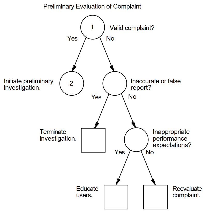 |
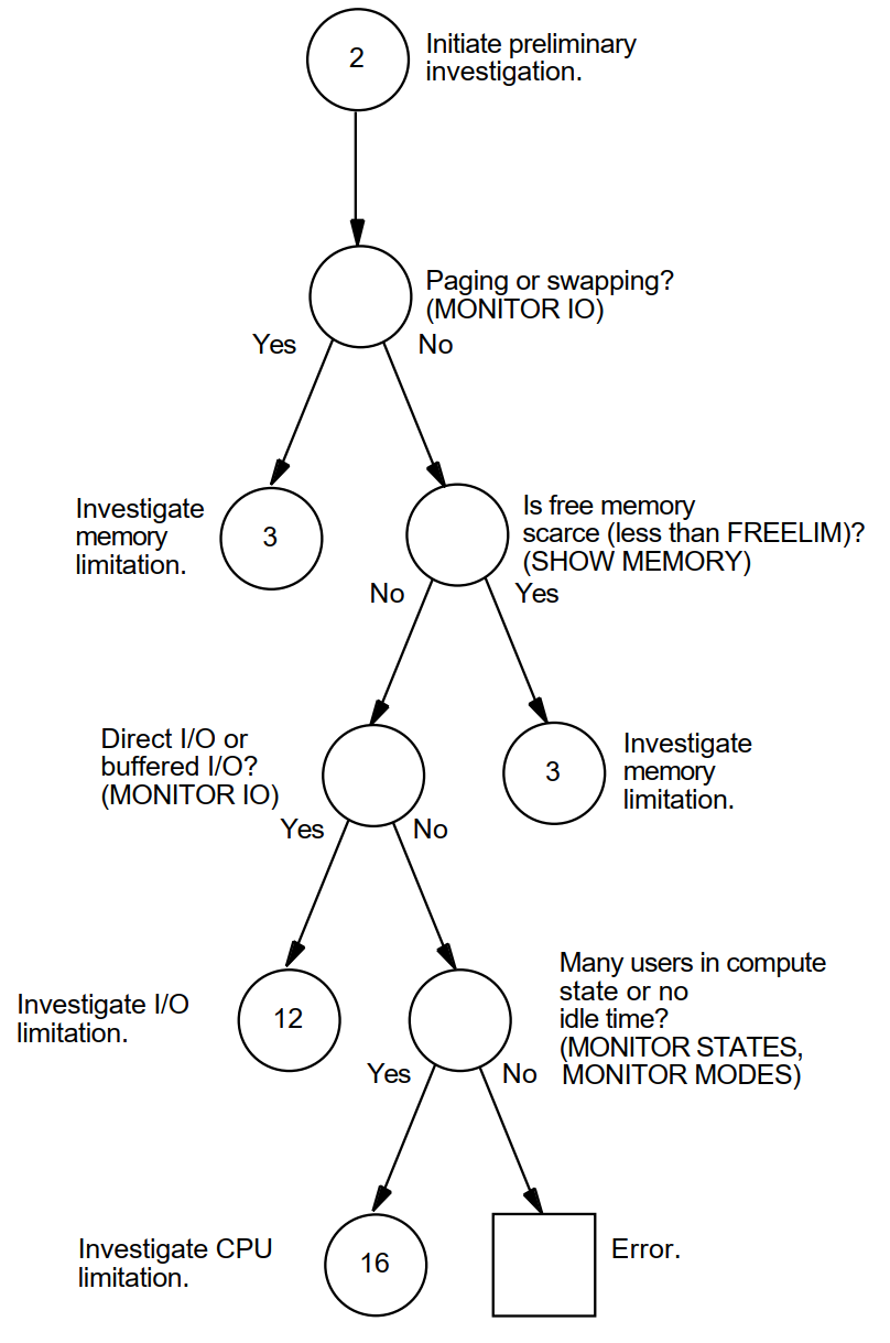 |
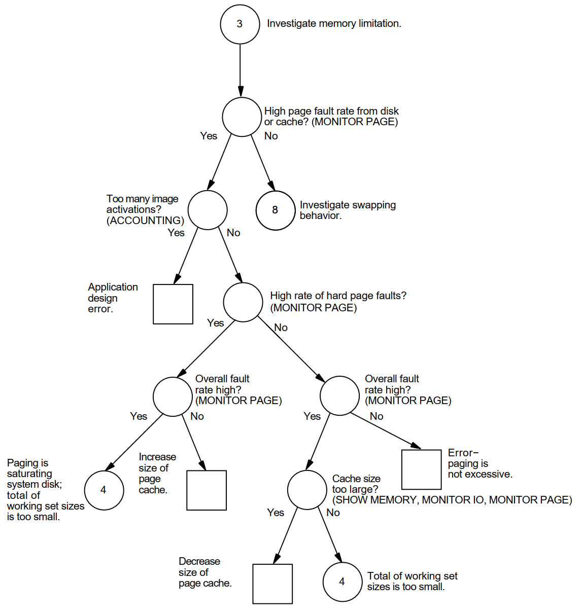 |
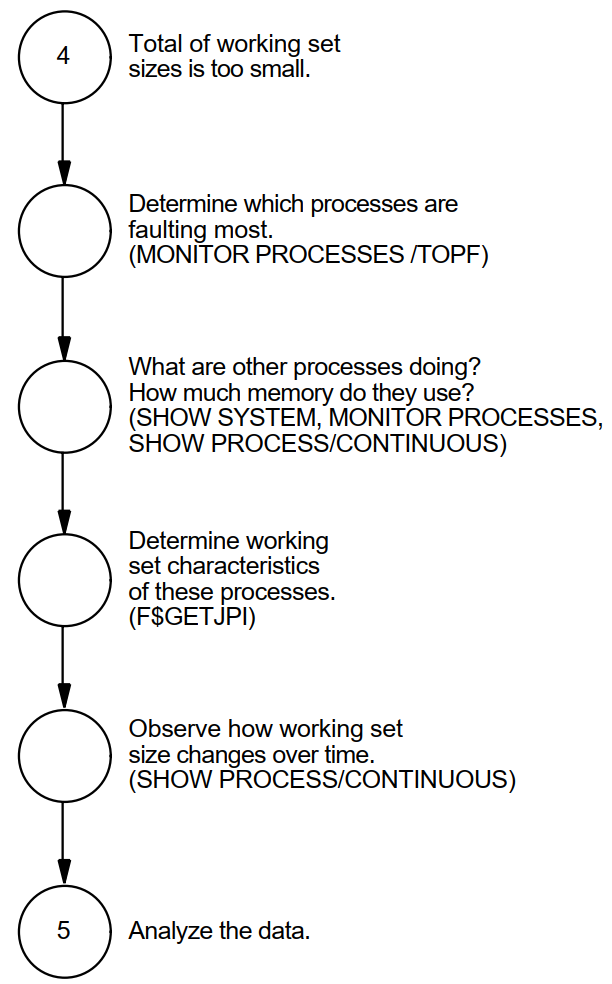
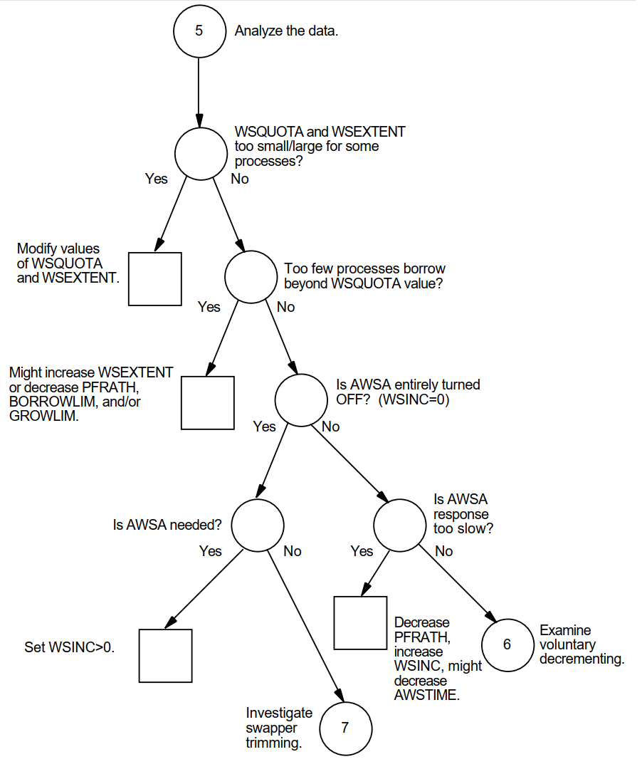 |
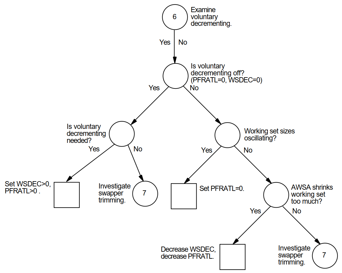 |
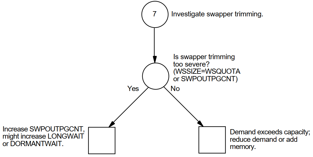 |
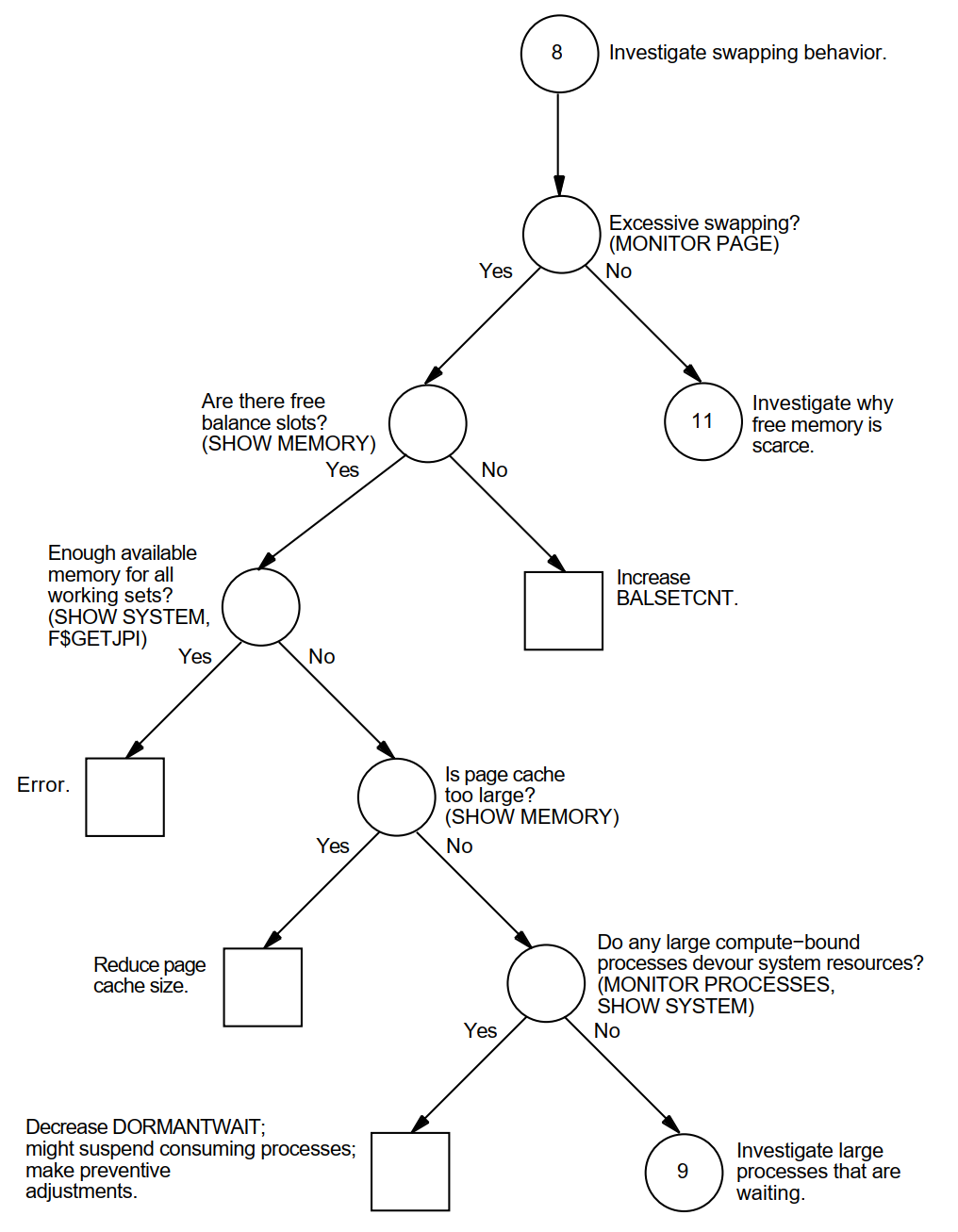 |
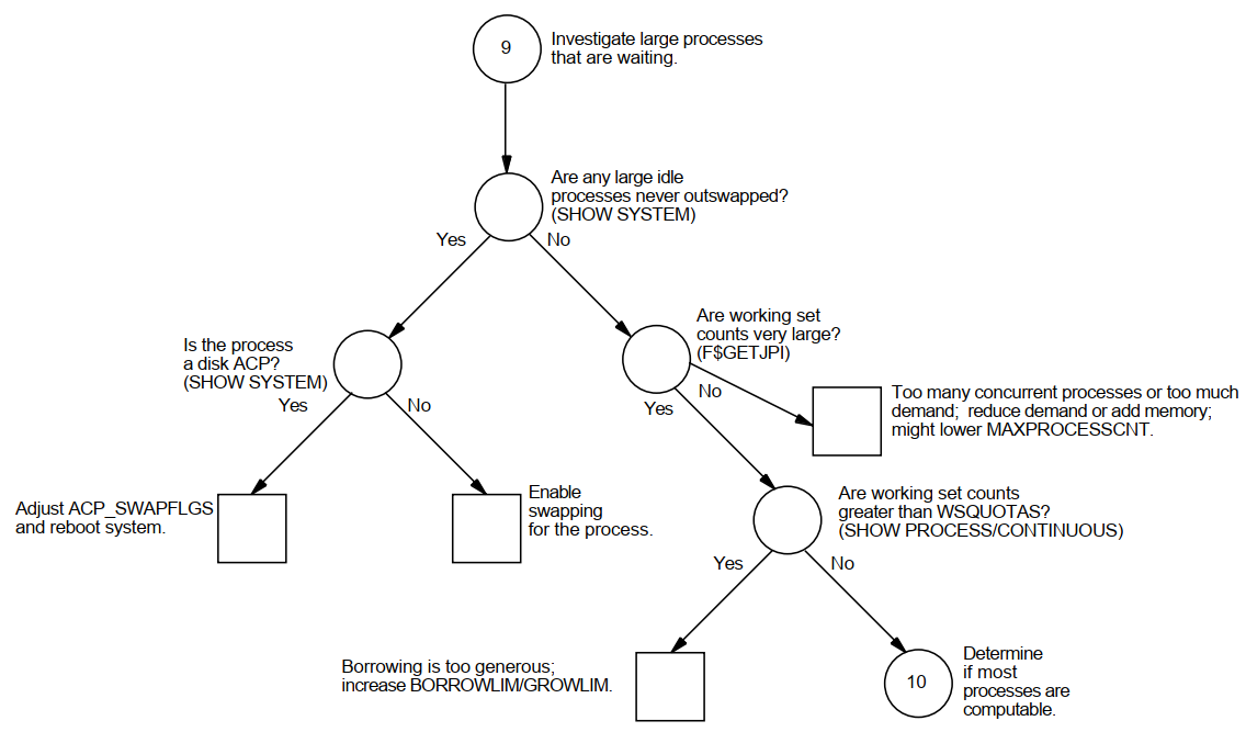 |
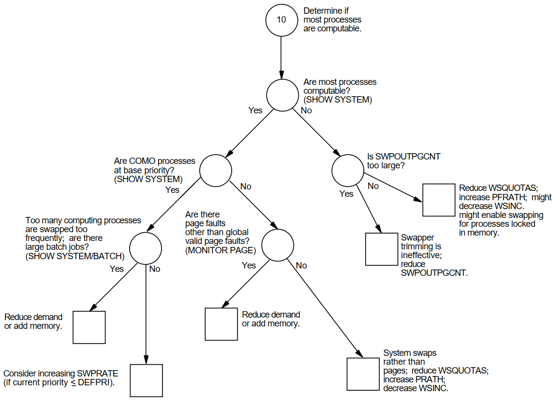 |
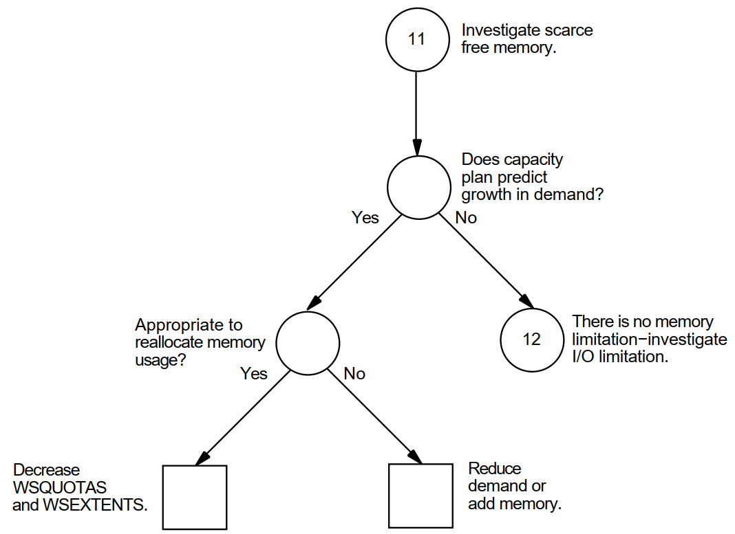 |
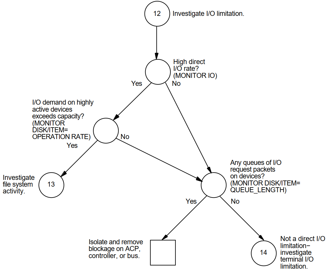 |
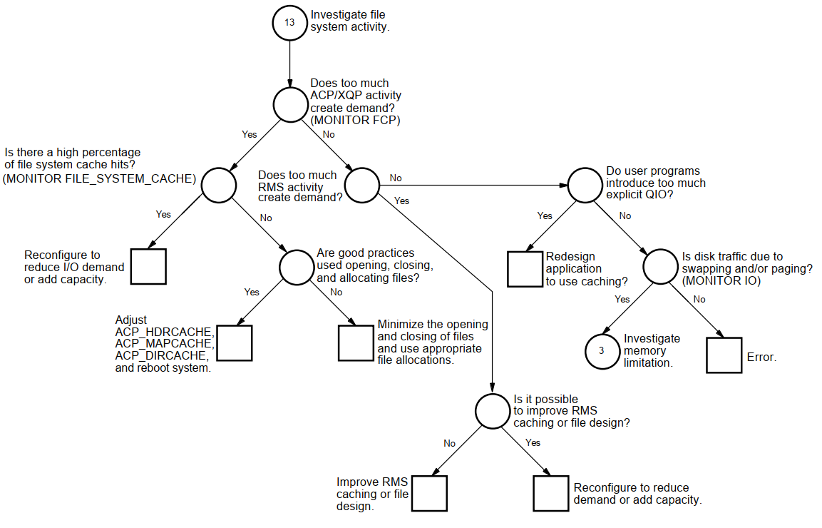 |
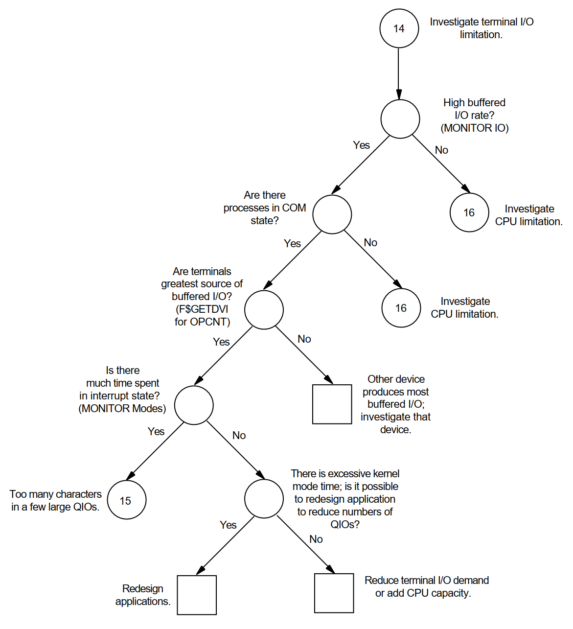 |
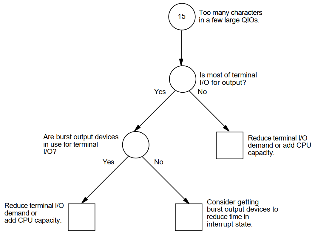 |
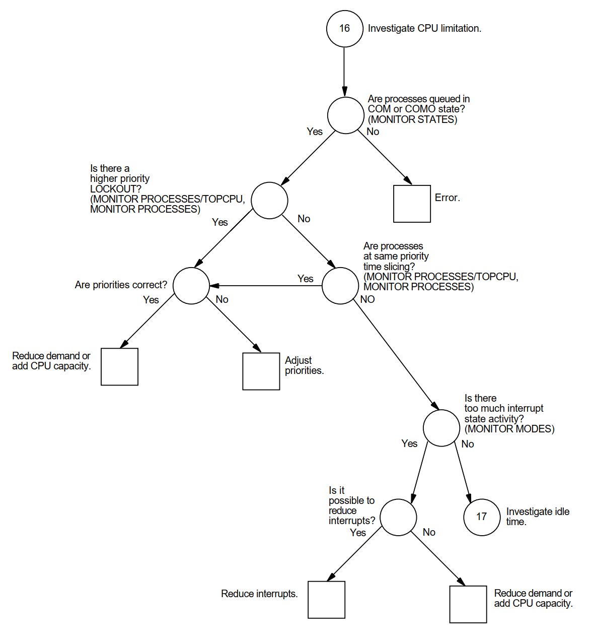 |
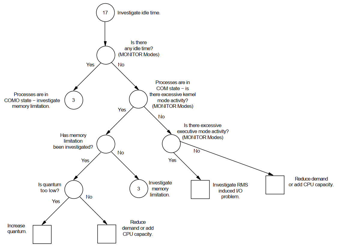 |
Appendix B. MONITOR Data Items
|
Item |
Class |
Description ? |
|---|---|---|
|
Compute Queue (COM + COMO) |
STATES |
Good measure of CPU responsiveness in most environments. Typically, the larger the compute queue, the longer the response time. |
|
Idle Time |
MODES |
Good measure of available CPU cycles, but only when processes are not unduly blocked because of insufficient memory or an overloaded disk I/O subsystem. |
|
Inswap Rate |
IO |
Rate used to detect memory management problems. Should be as low as possible, no greater than 1 per second. |
|
Interrupt State Time + Kernel Mode Time |
MODES |
Time representing service performed by the system. Normally, should not exceed 40% in most environments. |
|
MP Synchronization Time |
MODES |
Time spent by a processor waiting to acquire a spin lock in a multiprocessing system. A value greater than 8% might indicate moderate-to-high levels of paging, I/O, or locking activity. |
|
Executive Mode Time |
MODES |
Time representing service performed by RMS and some database products. Its value will depend on how much you use these facilities. |
|
Page Fault Rate |
PAGE |
Overall page fault rate (excluding system faults). Paging might demand further attention when it exceeds 600 faults per second. |
|
Page Read I/O Rate |
PAGE |
The hard fault rate. Should be kept below 10% of overall rate for efficient use of secondary page cache. |
|
System Fault Rate |
PAGE |
Rate should be kept to minimum, proportional to your CPU performance. |
|
Response Time (ms) (computed) |
DISK |
Expected value is 25–40 milliseconds for RA-series disks with no contention and small transfers. Individual disks will exceed that value by an amount dependent on the level of contention and the average data transfer size. |
|
I/O Operation Rate |
DISK |
Overall I/O operation rate. The following are normal load ranges
for RA-series disks in a typical timesharing environment, where the
vast majority of data transfers are small:
|
|
Page Read I/O Rate + Page Write I/O Rate + Inswap Rate (times 2) + Disk Read Rate + Disk Write Rate |
PAGE PAGE IO FCP FCP |
System I/O operation rate. The sum of these items represents the portion of the overall rate initiated directly by the system. |
|
Cache Hit Percentages |
FILE_SYSTEM_CACHE |
XQP cache hit percentages should be kept as high as possible, no lower than 75% for the active caches. |
Appendix C. MONITOR Multifile Summary Report
Figure C.1, ''Prime-Time OpenVMS Cluster Multifile Summary Report'', an OpenVMS Cluster prime-time multifile summary report, provides an extended context for the data items in Table B.1, ''Summary of Important MONITOR Data Items''.
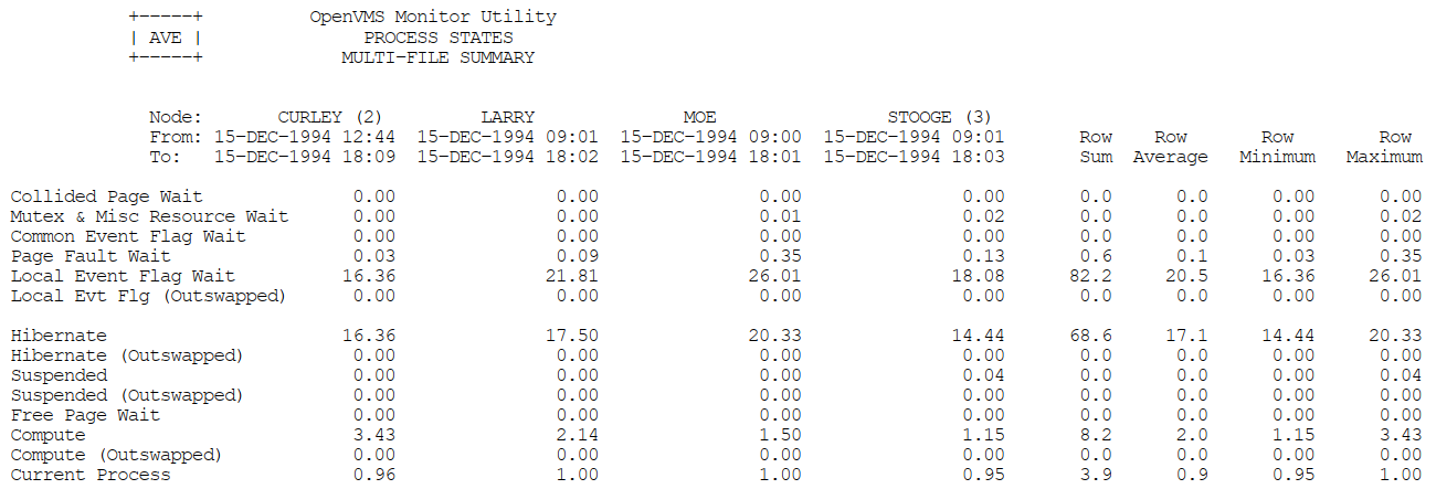 |
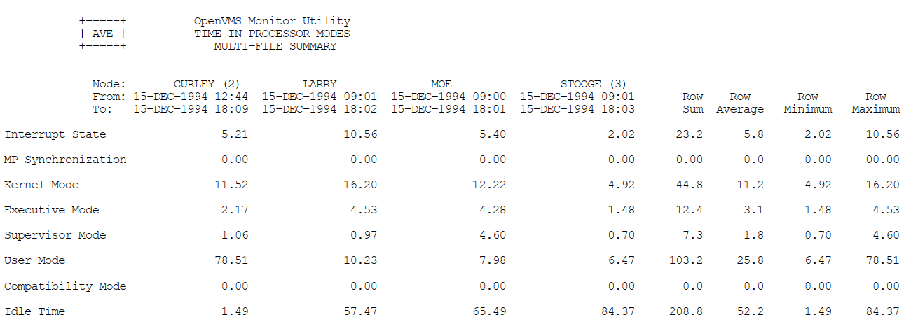 |
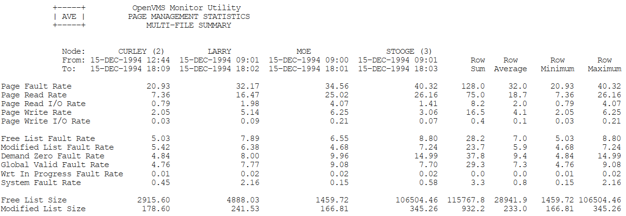 |
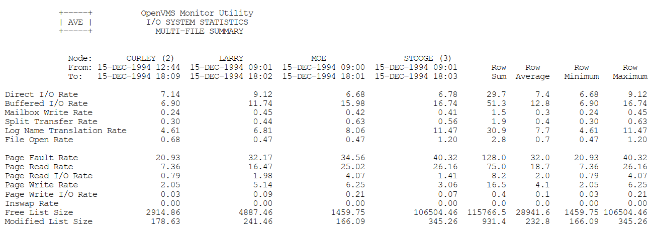 |
 |
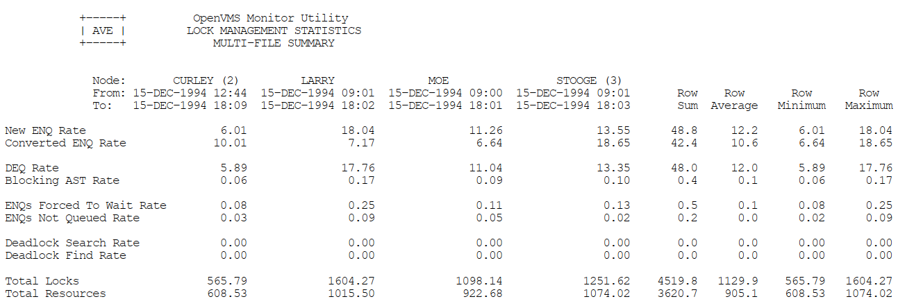 |
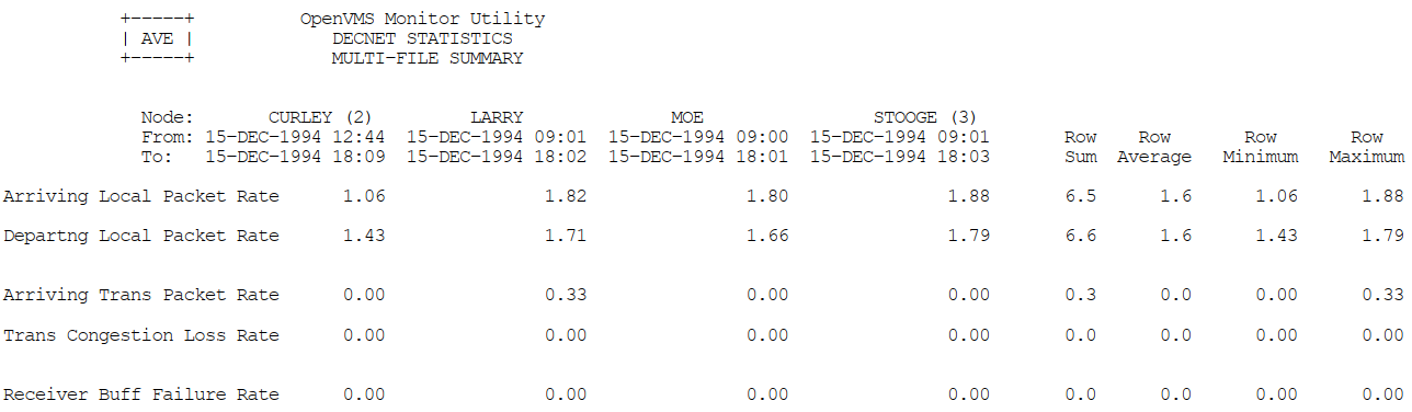 |
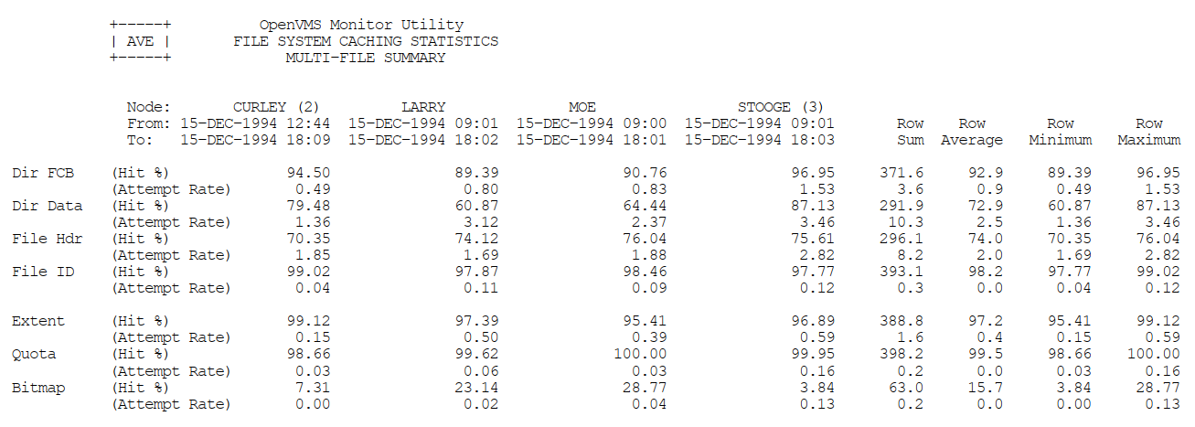 |
 |
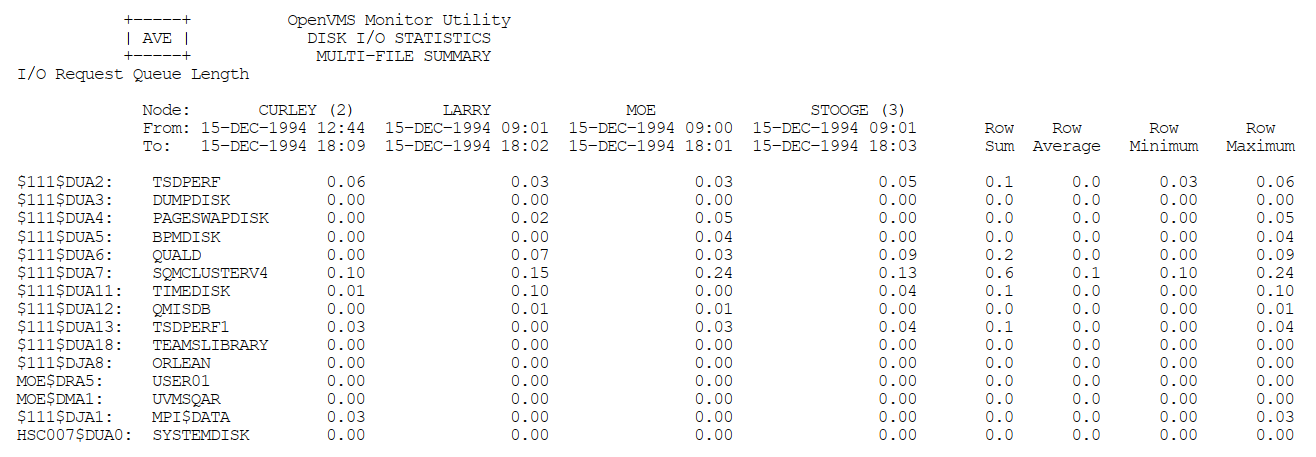 |
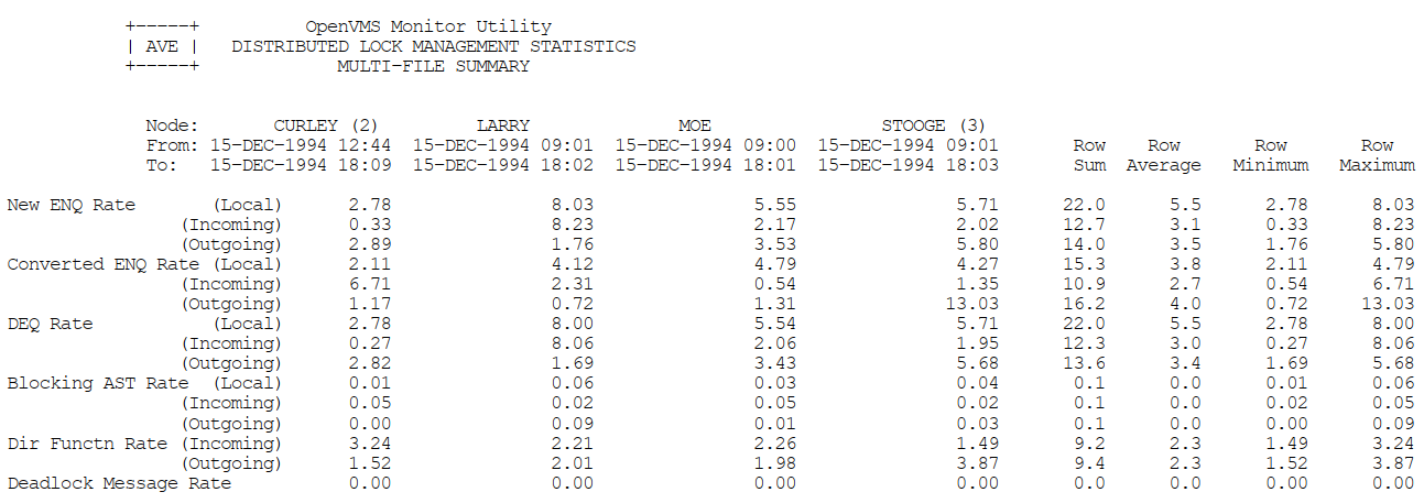 |
 |
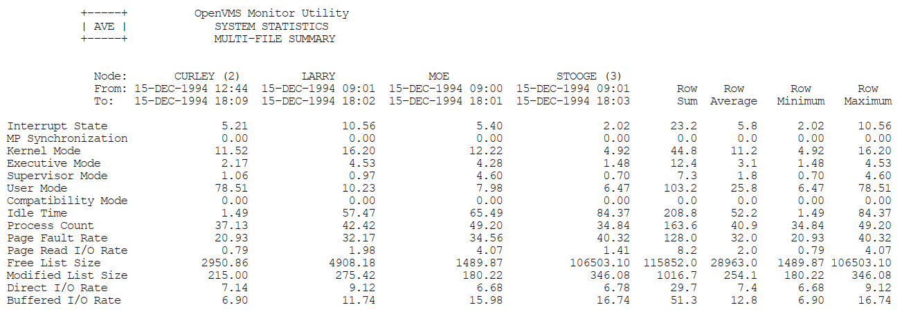 |
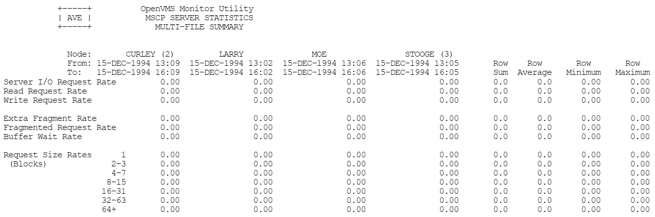 |
Appendix D. ODS–1 Performance Information
This appendix provides performance information specific to Files–11 ODS-1 (On-Disk Structure Level 1) disks.
D.1. Disk or Tape Operation Problems (Direct I/O)
Device I/O rate is below capacity.
Explicit QIO usage is too high.
D.1.1. Device I/O Rate Is Below Capacity
Sometimes you may detect a lower direct I/O rate for a device than you would expect. This condition implies that either very large data transfers are not completing rapidly (probably in conjunction with a memory limitation centered around paging and swapping problems) or that some other devices are blocking the disks or tapes.
If you have already investigated the memory limitation and taken all possible steps to alleviate it (which is the recommended step before investigating an I/O problem), then you should try to determine the source of the blockage.
A blockage in the I/O subsystem suggests that I/O requests are queueing up because of a bottleneck. For disks, you can determine that this condition is present with the MONITOR DISK/ITEM=QUEUE_LENGTH command.
When you find a queue on a particular device, you cannot necessarily conclude that the device is the bottleneck. At this point, simply note all devices with queues for later reference. (You will need to determine which processes are issuing the I/O operations for the devices with queues.)
As the next step, you should rule out the possibility of a lockout situation induced by an ancillary control process (ACP). Note that this condition arises only if you have ODS-1 disks. If the system attempts to use a single ACP for both slow and fast devices, I/O blockages can occur when the ACP attempts to service a slow device. This situation can occur only if you have mounted a device with the /PROCESSOR qualifier.
D.1.2. Explicit QIO Usage Is Too High
Next, you need to determine if any process using a device is executing a program that employs explicit specification of QIOs rather than RMS. If you enter the MONITOR PROCESSES/TOPDIO command, you can identify the user processes worth investigating. It is possible that the user-written program is not designed properly.
D.2. Adjust Working Set Characteristics: Establish Values for Ancillary Control Processes
An ancillary control process (ACP) acts as an interface between the user software and the I/O driver. The ACP supplements functions performed by the driver such as file and directory management.
Before studying the considerations for adjusting working set sizes for processes in general, consider the special case of the ACP. (Note that you will be using an ACP for disks only if you have ODS-1 disks.) The default size of the working set (and in this case, the working set quota, too) for all ACPs is determined by the system parameter ACP_WORKSET. If ACP_WORKSET is zero, the system calculates the working set size for you. If you want to provide a specific value for the working set default, you just specify the desired size in pages with AUTOGEN. (If your system uses multiple ACPs, remember that ACP_WORKSET is a systemwide parameter; any value you choose must apply equally well to all ACPs.)
If you decide to reduce ACP_WORKSET (with the intent of inducing modest paging in the ACP), use the SHOW SYSTEM command to determine how much physical memory the ACP currently uses. Set the system parameter ACP_WORKSET to a value that is 90 percent of the ACP's current usage. However, to make the change effective for all ACPs on the system, not just the ones created after the change, you must reboot the system.
Once you reduce the size of ACP_WORKSET, observe the process with the SHOW SYSTEM command to verify that the paging you have induced in the ACP process is moderate. Your goal should be to keep the total number of page faults for the ACP below 20 percent of the direct I/O count for the ACP.
D.3. Remove Blockage Due to ACP
Of the four sources of bottlenecks, the ACP lockout problem is the easiest to detect and solve. Moreover, it responds to software tuning.
Note that you will be using an ACP for disks only if you have ODS-1 disks.
The solution for an ACP lockout caused by a slow disk sharing an ACP with one or more fast disks requires that you dismount the slow device with the DCL command DISMOUNT, then enter the DCL command MOUNT/PROCESSOR=UNIQUE to assign a private ACP to the slow device. However, be aware that each ACP has its own working set and caches. Thus, creating multiple ACPs requires the use of additional memory.
Also, there are situations that might share some of the symptoms of an ACP lockout that will not respond to adding an ACP. For example, when substantial I/O activity is directed to the same device so that the activity in effect saturates the device, adding an ACP for another device without taking steps to redirect or redistribute some of the I/O activity to the other device yields no improvement.
D.3.1. Blockage Due to a Device, Controller, or Bus
When you are confronted with the situation where users are blocked by a bottleneck on a device, a controller, or a bus, first evaluate whether you can take any action that will make less demand on the bottleneck point.
D.3.2. Reduce Demand on the Device That Is the Bottleneck
If the bottleneck is a particular device, you can try any of the following suggestions, as appropriate. The suggestions begin with areas that are of interest from a tuning standpoint and progress to application design areas.
One of the first things you should determine is whether the problem device is used for paging or swapping files and if this activity is contributing to the I/O limitation. If so, you need to consider ways to shift the I/O demand. Possibilities include moving either the swapping or paging file (or both, if appropriate) to another disk. However, if the bottleneck device is the system disk, you cannot move the entire paging file to another disk; a minimum paging file is required on the system disk. See the discussion of AUTOGEN in the VSI OpenVMS System Manager's Manual, Volume 2: Tuning, Monitoring, and Complex Systems for additional information and suggestions.
Another way to reduce demand on a disk device is to redistribute the directories over one or more additional disks, if possible. You can allocate memory to multiple ACPs (ODS–1 only) to permit redistributing some of the disk activity to other disks. Section 12.4, ''Improve RMS Caching'' discusses RMS caching and some of the implications of using RMS to alleviate the I/O on the device. Also consider that, if the disks have been in use for some time, the files may be fragmented. You should run the Backup utility to eliminate the fragmentation. (See the VSI OpenVMS System Manager's Manual, Volume 1: Essentials.) If this approach is highly successful, institute a more regular policy for running backups of the disks.
As a next step, try to schedule work that heavily accesses the device over a wider span of time or with a different mix of jobs so that the demand on the device is substantially reduced at peak times. Moving files to other existing devices to achieve a more even distribution of the demand on all the devices is one possible method. Modifications to the applications may also help distribute demand over several devices. Greater changes may be necessary if the file organization is not optimal for the application; for example, if the application employs a sequential disk file organization when an indexed sequential organization would be preferable.
D.3.3. Reduce Demand on the Controller That Is the Bottleneck
When a controller is the bottleneck, balance the load by moving demand to another controller. If all controllers are overloaded, acquire additional hardware.
D.3.4. Reduce Demand on the Bus That Is the Bottleneck
Another suggestion is to place controllers on separate buses. Again, you want to segregate the slower speed units from the faster units.
When a bus becomes the bottleneck, the only solution is to acquire another bus so that some of the load can be redistributed over both buses.
Mount the disk on which it resides in SYLOGICALS.
When used with the DCL command START/QUEUE/MANAGER.
If MMG_CTLFLAGS equals 0, then active memory reclamation is disabled.
For example, if the event is the completion of terminal I/O input, the scheduler gives a large increase so that the process can run again sooner.
The priority is never decreased below the base priority or increased into the real-time range.
See the entries for Free List Size and Modified List Size.
See the Page Fault Rate.
See the Inswap Rate.
RMS and the XQP use locks to synchronize record and file access.
Note that the values of the parameters are not actually changed.
Setting POOLCHECK to a nonzero value overrides the settings imposed by SYSTEM_CHECK.
As a general rule, the combination of interrupt time and kernel mode time should be less than 40 percent of the total CPU time used.
The values and ranges of values shown are averages. They are intended only as general guidelines and will not be appropriate in all cases.